This section describes the basic statistical functions that come with Excel. To see which functions Excel provides or to see which arguments a function requires, click the Paste Function toolbar button and then select Statistical from the Function Category list box (see Figure 4-1).
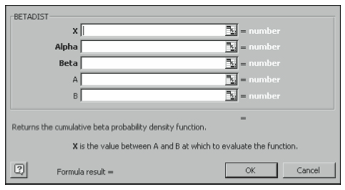
Once you select a function and click Next, the second Paste Function dialog box shows which arguments are required for the function to make its calculations (see Figure 4-2).
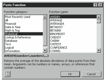
This chapter describes the statistical functions in a way that allows you to enter them directly in a cell without using the Paste Function dialog box. However, if you want to use the Paste Function dialog box, you just enter the arguments described in this chapter in the text boxes of the Paste Function dialog box.
Average Absolute Deviation from the Mean (AVEDEV)
The AVEDEV function finds the average of the absolute value of the deviation from the mean for each value in a data set. The AVEDEV function uses the following syntax:
=AVEDEV(data set range)
To use the AVEDEV function, simply enter the data set range as the single argument in the function. For example, if your data set is in the range A1:C10, you would enter the function as follows:
=AVEDEV(A1:C10)
Beta Probability Density
BETADIST
The BETADIST function returns the cumulative beta probability density function. Statisticians often use the cumulative beta probability density function to study variation across samples, such as when comparing two groups of people performing the same task to see whether they have the same success rate. The BETADIST function uses the following syntax:
=BETADIST(x,alpha,beta,A,B)
where x is a value between two optional bounds A and B, and alpha and beta are the two positive parameters. For example, if x equals 2, alpha equals 85, beta equals 90, A equals 1, and B equals 3, you would enter the function as follows:
=BETADIST(2,85,90,1,3)
The formula returns the value 0.647616.
BETAINV
The BETAINV function returns the inverse of the cumulative beta probability density function. That is, you use the BETADIST function if you know x and want to find the probability, and you use the BETAINV function if you know the probability and want to find x. The BETAINV function uses the following syntax:
=BETAINV(probability,alpha,beta,A,B)
Binomial Probability Distribution
The binomial distribution describes the outcome of a multi-step experiment, consisting of n identical trials, where each trial ends in either a success or a failure and the probability of a success p does not change from trial to trial. The trials must also be independent so that success in one trial does not affect the probability of success in another trial. The binomial random variable x is the number of successes observed in n trials.
BINOMDIST
For example, if you flip a coin n times and “heads” is called a success, then the random variable x would be the number of heads observed in n flips. It could take the values 1,2,3,…,n with different probabilities.
The BINOMDIST function uses the following syntax:
=BINOMDIST(x,n,p,cumulative)
If you want to find the probability of exactly x successes, enter FALSE as the fourth (cumulative) argument. If you want to find the probability of x or fewer successes, enter TRUE as the fourth argument.
For example, if you were to flip a fair coin 20 times and wanted to find the probability of it turning up “heads” exactly 10 times, the function looks like this:
=BINOMDIST(10,20,0.5,FALSE)
The function returns the value 0.176197052. If you wanted to find the probability of getting 10 or fewer heads, you replace the FALSE with TRUE, and the function returns the value 0.588098526.
Figure 4-3 shows another example of this function. For this example, suppose you know that 35% of your customers are women and you select 10 customers at random. What is the probability that you won’t select a woman? (In this case, it doesn’t matter whether you choose TRUE or FALSE as the cumulative argument, as there are no possible outcomes less than zero.)
CRITBINOM
The acceptance criterion function, CRITBINOM, is used for quality control of a production process. You use this function to find the maximum number of defective items that a person can find in a lot and still allow acceptance of the lot. Inspectors should accept the lot if they find this number or fewer defective items and reject the lot if they find more defective items.
To determine the acceptance criterion, you need to know the number of items in the lot, the probability of accepting each item, and the producer’s allowable risk (alpha) for rejecting an acceptable lot.
The CRITBINOM function uses the following syntax:
=CRITBINOM(trials,probability_s,alpha)
where trials is the number of trials, probability_s is the probability of a success on each trial, and alpha is the criterion value. Probability_s and alpha are both between 0 and 1.
NEGBINOMDIST
If the number of successes is fixed in a binomial distribution and you want to find the number of trials, use the NEGBINOMDIST function. This function returns the probability that there will be a certain number of failures before the threshold number of successes, given the constant probability of a success.
For example, if you need to find 20 straight 2 by 4s from a stack, and you know the probability that a board in the stack is straight is 0.2 (20%), you can use the NEGBINOMDIST to find that there is about a 2% probability that you will reject 75 boards before finding all 20 straight ones.
The NEGBINOMDIST function uses the following syntax:
=NEGBINOMDIST(number failures,number successes,probability of success)
For this example, the function looks like this:
=negbinomdist(75,20,0.2)
Chi-Square Distribution
The chi-square distribution is commonly used to make inferences about a population variance. If a population follows the normal distribution, you can draw a sample of size N from this distribution and form the sum of the squared standardized scores (chi-square). This random variable chi-square follows the chi-square probability distribution with n degrees of freedom (df ), where n is a positive integer equal to N-1. The degrees of freedom parameter determines the shape of the distribution. With more degrees of freedom, the skew is less.
CHIDIST
The CHIDIST function returns the area in the upper tail of the chi-square distribution. You use the CHIDIST function the same way you would use a chi-square distribution table. The CHIDIST function uses the following syntax:
=CHIDIST(x,df)
For example, if you pull a random sample of 16 from a population and want to find the probability of a sample chi-square value (x) 25 or larger, you would enter:
=CHIDIST(25,15)
The function returns the value 0.049943, meaning that a value of 25 or more should in the long run occur about five times in a hundred.
CHIINV
You can use the CHIINV function to create confidence interval estimates of a population variance. That is, you use the CHIDIST function if you know x and want to find the probability, and you use the CHIINV function if you have a probability and want to find x. For example, if you’re creating a product and weigh a sample of 18 units to find a sample variance of 0.36, you may want to construct a 90% confidence interval estimate of the population variance for the product. With a sample size of 18, you have 17 degrees of freedom. To find the upper limit, enter:
=CHIINV(0.95,17)
To find the lower limit, enter:
=CHIINV(0.05,17)
These formulas return the values 8.67175 and 27.5871. Multiply the sample variance of 0.36 by the degrees of freedom and divide this product by each of the values returned from the CHIINV function to find the lower and upper limits of the confidence interval. You can take the square root of these values to establish interval estimates of the population standard deviation.
CHITEST
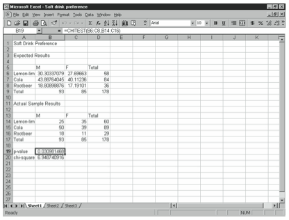
The chi-square test is used to test independence of two variables. You can use the chi-square test to determine whether there is a significant difference between observed and expected frequencies. For example, if you want to find out whether soft drink preference differs between male and female drinkers, you can construct a null hypothesis that soft drink preference is independent of the gender of the drinker, and create a table of expected results based on a sample of 93 male drinkers and 85 female drinkers as shown in Figure 4-4. You can then create a table of the results of the actual study findings.
The CHITEST formula uses the following syntax:
=CHITEST(actual range,expected range)
where actual range is the data in the actual sample results table and expected range is the data from the expected results table. In the example shown in Figure 4-4, cell B19 contains the following formula:
=CHITEST(B6:C8,B14:C16)
The formula returns the value 0.03098. This is the p-value. You reject the null hypothesis if this value is less than your level of significance alpha. So if your level of significance is .05, you would reject it, but not if your level of significance is .025 or .01.
Confidence Intervals for Population Means (CONFIDENCE)
A confidence interval is the interval around a sample mean into which you expect the population mean to fall a certain percentage of the time. If you have a sample of size n and know the sample mean m and population standard deviation sigma (s), you can find the range into which the actual population mean will fall x% of the time. Common confidence levels are 90%, 95%, and 99%. The CONFIDENCE function uses the following syntax:
=CONFIDENCE(alpha,s,n)
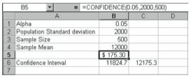
For example, if a sample of 500 college graduates shows that they owe an average of $12,000 in student loans at graduation and the population standard deviation is $2,000, you can find a 95% confidence interval estimate of the population mean amount owed. To do this using the CONFIDENCE function, enter alpha .05 as the first argument, the standard deviation 2000 as the second argument, and n 500 as the third argument. The function looks like this:
=CONFIDENCE(0.05,2000,500)
The function returns the value 175.30. So you can say with 95% confidence that the population mean is $12,000 plus or minus $175.30. Figure 4-5 illustrates this calculation.
Correlation
Correlation shows the closeness of the relationship between two variables. The benefit of using a correlation coefficient to measure the relationship between two variables as opposed to using covariance is that the unit of measurement doesn’t matter.
CORREL
You use the CORREL function in Excel to determine whether two data sets are related, and if so, how strongly. The correlation coefficient ranges from +1, indicating a perfect positive linear relationship, to –1, indicating a perfectly negative linear relationship. To calculate a correlation coefficient for a sample, Excel uses the covariance of the samples and the standard deviations of each sample. To use the CORREL function in Excel, just select the two sets of data to use as the arguments and use the following syntax:
=CORREL(data set 1,data set 2)
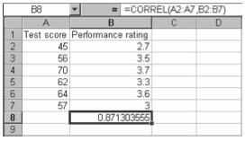
For example, if you have a set of preliminary test scores for a sample of employees in column A and a set of performance feedback scores in column B, as shown in Figure 4-6, and you want to find out whether they’re related and if so, how strongly, you can use Excel to find the correlation coefficient for the samples.
The function returns the value 0.87, indicating that the sets are positively related (as the value of one goes up, the value of the other also increases), but the relationship isn’t perfect.
PEARSON
The Pearson product moment correlation coefficient function, PEARSON, uses a different equation for calculating the correlation coefficient. This formula doesn’t require the computation of each deviation from the mean. Still, the correlation coefficient ranges from +1, indicating a perfect positive linear relationship, to –1, indicating a perfectly negative linear relationship. The PEARSON function uses the following syntax:
=PEARSON(data set 1,data set 2)
Using the PEARSON function on the data shown in Figure 4-6 to compute the correlation coefficient returns the same value as the CORREL function does.
RSQ
The RSQ function calculates the square of the Pearson product moment correlation coefficient through data points in the data sets. You can interpret the r-squared value as the proportion of the variance in y attributable to the variance in x. The RSQ function uses the following syntax:
=RSQ(data set 1,data set 2)
Counting Cells
If you select a range of cells, you can have Excel find how many cells are in that range using the count functions.
COUNT
To find the number of cells in a range that contain numbers (or dates, or textual representations of numbers), you use the COUNT function. This function does not count cells containing text or logical values like TRUE and FALSE, nor does it count empty cells. The COUNT function uses the following syntax:
=COUNT(data set range)
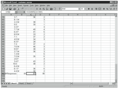
For example, if you have a database of 100 customer survey responses, and column C contains numeric responses to the question if a customer chose to respond, you can find out how many people answered the question using the COUNT function, as shown in Figure 4-7.
COUNTA
The COUNTA function counts all cells in a range that aren’t empty, including cells with error values, logical values, and text. The COUNTA function uses the following syntax:
=COUNTA(data set range)
COUNTBLANK
The COUNTBLANK function counts only blank cells. The COUNTBLANK function uses the following syntax:
=COUNTBLANK(data set range)
COUNTIF
The COUNTIF function counts the cells that fit the criteria you specify. The COUNTIF function uses two parameters, the data set range and the condition, in the following syntax:
=COUNTIF(data set range,condition)
For example, if you want to count cells that exactly match a number or value, just enter that number or value. To count cells that are greater than or less than a value, use the symbols >, >=, <, and <= followed by the value. If you are using any of these symbols, you need to put the condition in quotes. For example, if you want to know how many numbers in cells A1:C5 are greater than one, you would use the following function:
=COUNTIF(A1:C5,”>1″)
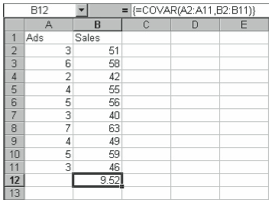
A positive correlation coefficient, as shown in this example, indicates a positive relationship, that is, as the number of advertisements increases, the number of sales increases. Note, however, that a large positive value does not indicate a strong positive linear relationship, nor does a large negative value indicate a strong negative linear relationship. The value you obtain for covariance depends on the units of measurement you use. For example, if you want to test the relationship between weight and volume, you would obtain different values for covariance depending on whether you used ounces or grams, cubic inches or cubic centimeters.
Exponential Probability Distribution (EXPONDIST)
To describe the time it takes to complete a task, you use the exponential probability distribution, EXPONDIST. For example, you can describe the time between arrivals of vehicles in a drive-through or the time required to load a crate of goods. Product lifetimes also often follow an exponential probability distribution. For example, if the average lifetime of a part in a machine is 15 years, you can find the probability that the part will last less than a certain number of years, more than a certain number of years, or between numbers of years. The EXPONDIST function uses the following syntax:
=EXPONDIST(x,lambda,cumulative)
where lambda is the inverse of the mean and cumulative allows you to tell Excel whether you want the cumulative probability or the probability of exactly that value.
For example, if you want to find the probability that a part with a mean lifetime of 12 years lasts less than 6 years, enter the function as follows:
=EXPONDIST(6,1/12,TRUE)
The function returns the value 0.3935.
Exponential Regression
Exponential regression finds the equation of an exponential equation of the form y = abx that best fits a data set.
LOGEST
The LOGEST function calculates an exponential curve that best fits your data and returns an array that describes the curve. The LOGEST function uses the following syntax:
=LOGEST(known ys,known xs,constant,statistics)
If the constant is set to False, b is set to be equal to 1. If statistics is set to True, you get an array of additional data on the error in the value of the coefficients.
GROWTH
You can use the GROWTH function in two ways: to calculate predicted exponential growth for a series of new x-values using existing x-values and y-values, or to fit an exponential curve to existing x-values and y-values. The GROWTH function uses the following syntax:
=GROWTH(known y’s,known x’s,new x’s,constant)
If the constant is set to False, b is set to be equal to 1.
F Probability Distribution
If you want to compare the variances of two normal populations using data collected from two independent random samples of size N(1) and N(2) of these populations,it results in an F distribution with N(1)-1 degrees of freedom and N(2)-1 degrees of freedom.
FDIST
If you know a value and want to find the probability in the F distribution, you use the FDIST function. The FDIST function uses the following syntax:
=FDIST(x,degrees of freedom 1,degrees of freedom 2)
FINV
If you know the probability and want to find a value for the F distribution, you use the FINV function. The FINV function uses the following syntax:
=FINV(probability,degrees of freedom 1,degrees of freedom 2)
FTEST
The F-test finds the one-tailed probability that the variances in two data sets are not significantly different. For example, scientists use the F-test to compare pairs of data obtained from particular laboratories, analysts, or methods to determine whether one batch is significantly more precise than the other. The FTEST function uses the following syntax:
=FTEST(array 1,array 2)
Fisher Transformation
The Fisher’s z’ transformation converts Pearson’s r to the normally distributed variable z’. You use the Fisher’s z’ to compute confidence intervals on Pearson’s correlation and on the difference between correlations.
FISHER
The FISHER function computes from r to z’. The function has the following syntax:
=FISHER(r)
FISHERINV
The FISHERINV function computes from z’ to r. The function has the following syntax:
=FISHERINV(z?)
Frequency (FREQUENCY)
The FREQUENCY function calculates how often values occur within a range of values, and then returns a vertical array of numbers. For example, use FREQUENCY to count the number of test scores that fall within ranges of scores. Because FREQUENCY returns an array, you must enter it as an array formula. The frequency formula uses the following syntax:
=FREQUENCY(data array,bins array)
where data array is an array of values for which you want to count frequencies and bins array is an array of bins (listed in ascending order and as upper limits) into which you want to group the values in the data array.
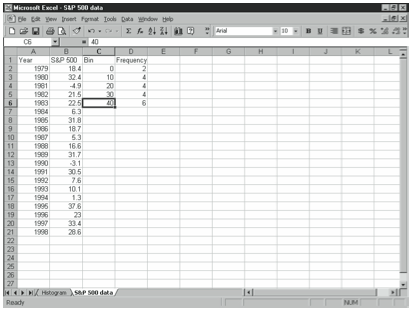
For example, if you wanted to create a frequency distribution using the S&P 500 data and bins shown in Figure 4-9, you would select the range D2:D6, enter:
=FREQUENCY(B2:B21,C2:C6)
and press Ctrl+Shift+Enter. When Excel constructs the frequency distribution, it counts the number of items with values less than or equal to the upper limit of the each bin, and and 6 in the corresponding cells.
Gamma Probability Distribution
If a Poisson process produces successes at a constant rate of m per unit of time, then the random variable x, the elapsed time until the rth success, follows the gamma distribution. The gamma distribution is often used to determine the amount of time it takes for the rth person to arrive in a line.
GAMMADIST
If you know x and want to find the probability, you use the GAMMADIST function, which has the following syntax:
=GAMMADIST(x,alpha,beta,cumulative)
For example, if x equals 25, alpha equals 8, beta equals 9, and cumulatative is TRUE, you use the following formula:
=GAMMADIST(25,8,9,TRUE)
The function returns the value 0.007774.
GAMMAINV
If you have been given a probability and want to find x, you use the GAMMAINV function, which has the following syntax:
=GAMMAINV(probability,alpha,beta)
For example, if the probability equals .5, alpha equals 8, and beta equals 9, you use the following formula:
=GAMMAINV(.5,8,9)
The function returns the value 69.02.
GAMMALN
You use the GAMMALN function to find the natural logarithm of the gamma function, G(x). The GAMMALN function uses the following syntax:
=GAMMALN(x)
For example, if x equals 25, you use the following formula:
=GAMMALN(25)
The function returns the value 54.78.
Geometric Mean (GEOMEAN)
If you have a set of n numbers, the geometric mean of the set is the nth root of the product of the numbers. To find the geometric mean, enter the data set range as the sole parameter of the GEOMEAN function, which uses the following syntax:
=GEOMEAN(data set range)
Harmonic Mean (HARMEAN)
The harmonic mean is the reciprocal of the mean of the reciprocals of a data set. To find the harmonic mean, enter the data set range as the sole parameter of the HARMEAN function, which uses the following syntax:
=HARMEAN(data set range)
Hypergeometric Distribution (HYPGEOMDIST)
The hypergeometric probability distribution is much like the binomial probability distribution. The hypergeometric distribution describes the outcome of a multi-step experiment, consisting of n trials, where each trial ends in either a success or a failure. But unlike the binomial distribution, the trials are not independent—so success in one trial affects the probability of success in another trial and the probability of success changes from trial to trial. The HYPGEOMDIST is therefore used when samples are taken from a finite population but not replaced for the next trial. The HYPGEOMDIST function uses the following syntax:
=HYPGEOMDIST(successes_in_sample,sample_size,number_of_successes,population)
For example, suppose a shipment of 10 items has 2 defective items and 8 nondefective items. If you randomly select and test the individual units and set aside the units you’ve tested, the probability of finding a defective unit changes depending on what’s left in the shipment. Suppose that you must reject a shipment if you find a single defective unit. If you sample 3 items, what’s the probability that the shipment will be accepted? To find out, you can call finding a defective item a “success,” and enter the HYPGEOMDIST function to look like this:
=HYPGEOMDIST(0,3,2,10)
This means 0 “successes” in 3 trials when there are 2 “successes” in the population of 10. The function returns the value 0.4667.
Theprobabilityofrejectingtheshipmentis1–0.4667,or0.5333.Toverifythis,youcanadd the probability of getting 1 success with the probability of having 2 successes.
Kurtosis (KURT)
Kurtosis is used to help determine the size of the tails in a distribution. The kurtosis of a normal distribution is 0. A negative kurtosis value means that a distribution has smaller tails than the normal curve, a positive kurtosis indicates a distribution with larger tails than the normal curve. The KURT function uses the following syntax:
=KURT(data set range)
Linear Regression
You use linear regression functions to find a linear equation that best describes a data set. Excel uses the sum of least squares method to find the straight line of best fit. People often try to predict future amounts by assuming linear growth and extending the line forward in time. For example, if you have a series of sales data for 9 months and want to predict the sales in the 10th month, you can use Excel’s linear regression functions to find the slope and y-intercept (the point on the y-axis where the line crosses) of the line that best fits the data.
To use the linear regression functions, it helps to remember the equation for a line:
y=mx+b
where y is the dependent variable, m the slope, x the independent variable, and b the y-intercept. If there are multiple ranges of x values, the equation looks like this:
y=m(1)x(1) +m(2)x(2) +…m(n)x(n) + b
FORECAST
The FORECAST function predicts a future y-value for the x-value you specify using existing x and y values. The FORECAST function uses the following syntax:
=FORECAST(x,known ys,known xs)
where x is the x-value for which you want to predict a y-value.
INTERCEPT
If you have existing x and y values, Excel can find the straight line that best fits the data and then calculate the point at which the line intersects the y-axis, in other words, the value of b in the “y=mx+b” equation. The y-intercept is useful when you want to know the value of the dependent variable when the independent variable equals 0.
The INTERCEPT function uses the following syntax:
=INTERCEPT(known ys,known xs)
LINEST
The LINEST function returns the value of m and b given at least one set of known ys and known xs. The LINEST function has the following syntax:
=LINEST(known ys,known xs,constant,statistics)
where known ys is the array of y values you already know, known xs is the array of x values you may already know. If you leave out the known xs, they are assumed to be 1, 2, 3,…n. If constant is set to FALSE, b is assumed to be 0. If statistics is set to TRUE, the LINEST function also returns the standard error for each data point.
SLOPE
Use the SLOPE function to find the slope (m) of the linear regression line from the known x and known y data sets. The slope is the change in y over the change in x for any two points on the line. The SLOPE function in Excel uses the following syntax:
=SLOPE(known ys,known xs)
A positive (upwards) slope means that the independent variable (such as the number of salespeople) has a positive effect on a dependent variable (such as sales). A negative (downwards) slope means that the independent variable has a negative effect on the dependent variable. The steeper the slope, the more effect the independent variable has on the dependent variable.
STEYX
Use the STEYX function to find the standard error of the predicted y-value for each individual x in the regression. The STEYX function uses the following syntax:
=STEYX(known ys,known xs)
TREND
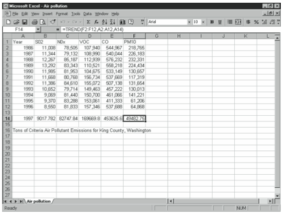
Use the TREND function to find values along a linear trend. Specify an array of new xs and the TREND function uses the method of least squares to fit a straight line to the known x and y data sets and return the y-values along the line for the new array. If constant is set to FALSE, the “b” in the y=mx+b equation is set to zero. The TREND function uses the following syntax:
=TREND(known ys,known xs,new xs,constant)
For example, in the worksheet of air pollutant values from 1986 to 1996 shown in Figure 4-10, you can predict air pollutant values for 1997 (assuming they follow a linear equation).
Lognormal Distribution Function
The lognormal distribution occurs when the natural logarithm of a random variable follows the normal distribution. People commonly assume that prices for stocks and Treasury bonds are lognormally distributed, that is, that returns for these investments are normally distributed.
LOGNORMDIST
Use the LOGNORMDIST function on data that has been logarithmically transformed to find the cumulative lognormal distribution of x, where ln(x) is normally distributed around the mean with a specific standard deviation. The LOGNORMDIST function uses the following syntax:
=LOGNORMDIST(x,mean,standard deviation)
where x is the value at which you want to find the function.
LOGINV
If you know the probability and want to find the value x, you use the inverse of the lognormal cumulative distribution function, LOGINV. The LOGINV function uses the following syntax:
=LOGINV(probability,mean,standard deviation)
Maximums and Minimums
Excel provides four functions for finding the maximum and minimum values in a data set.
MAX
The MAX function returns the largest value in a set of data. It ignores blank cells and cells containing text or logical values such as TRUE and FALSE. The MAX function uses the following syntax:
=MAX(data set range)
MAXA
The MAXA function returns the largest value in a set of data, but it includes logical values and text. It counts TRUE as 1 and FALSE and all other text as 0. The MAXA function uses the following syntax:
=MAXA(data set range)
MIN
The MIN function returns the smallest value in a set of data. It ignores blank cells and cells containing text or logical values such as TRUE and FALSE. The MIN function uses the following syntax:
=MIN(data set range)
MINA
The MINA function returns the smallest value in a set of data, but it includes logical values and text. It counts TRUE as 1 and FALSE and all other text as 0. The MINA function uses the following syntax:
=MINA(data set range)
Mean
Excel provides two functions for finding the mean of a data set. Both take the sum of the values in the set and divide it by the number of values.
AVERAGE
The AVERAGE function ignores cells that contain text, that are empty, or that contain logical values. To use the AVERAGE function, simply enter the data set range as the single argument using the following syntax:
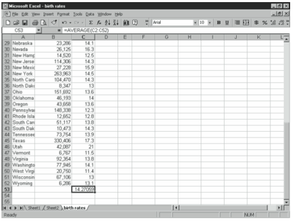
=AVERAGE(data set range)
For example, if you wanted to find the average birth rate per 1,000 people in the United States in 1996 using the data in Figure 4-11, you would use the following formula:
=AVERAGE(C2:C52)
The function returns the value 14.27.
AVERAGEA
The AVERAGEA function includes cells containing text or logical values in the calculation. Excel includes cells containing the word TRUE as the value 1 in the calculation; it includes cells containing the word FALSE or any other text as the value 0.
To use the AVERAGEA function, simply enter the data set range as the single argument in the function using the following syntax:
=AVERAGEA(data set range)
Median (MEDIAN)
The median is the middle value in a set of values. Half of the data in the set fall above this value and half fall below, so the median estimates the 50% quantile. The MEDIAN function uses the following syntax:
=MEDIAN(data set range)
If the data set contains an even number of values, Excel averages the two middle values.
Mode (MODE)
The mode is the most-frequently occurring value in a set of values. When Excel calculates the mode, it ignores empty cells and cells containing text or logical values. The MODE function uses the following syntax:
=MODE(data set range)
Normal Probability Distribution
The normal, or Gaussian, probability distribution has a bell-shaped curve. It is characterized by its mean mu (µ) and standard deviation sigma (s). The mean describes the location of the curve, the standard deviation describes the shape (how peaked or flat it is). The mean, the median, and the mode are all equal in a normal distribution.
NORMDIST
If you have a normal distribution and know the mean and standard deviation, you can find the probability that a random variable x falls below a given value using the NORMDIST function. The NORMDIST uses the following syntax
=NORMDIST(x,mean,standard deviation,cumulative)
For example, if containers are filled with an average of 591 ml of liquid, and the volumes are normally distributed around this mean with a standard deviation of 3 ml, you can find the probability that a container has less than 586 ml of liquid. To do this, enter 586 for the first parameter x, 591 for the second parameter, 3 for the third parameter, and TRUE for the fourth parameter. The function looks like this:
=NORMDIST(586,591,3,TRUE)
The function returns the value 0.0477. So there’s about a 4.8% chance that a container holds less than 586 ml. You can find the probability that a value falls between a certain range by making a few simple calculations, remembering that there’s a 0.5 probability that a value falls on each side of the mean. For example, if you want to find the probability that a container holds between 585 and 593 ml of liquid, you find the probability that it contains less than 585 and subtract this from 0.5. Then you find the probability that it contains less than 593 and subtract 0.5. Then you add these two figures.
NORMINV
If instead of having a value and needing to find the probability that a random variable falls below it, you know the probability for the range into which a random variable must fall and need to find the value defining this range, you can use the NORMINV function. The NORMINV function uses the following syntax:
=NORMINV(probability,mean,standard deviation)
Using the previous example for the NORMDIST function, if the mean fill volume in a set of containers is 591ml with a standard deviation of 3ml, and you want to be able to say that there’s a 99% probability of a container holding more than a certain volume of fluid (i.e., you want to find an amount below which the area under the curve is 0.01), enter the function as follows:
=NORMINV(0.01,591,3)
The function returns the value 584.02, meaning that there’s a 1% probability of a container filled with less than this amount.
Permutations (PERMUT)
When you select a sample from a population and the order of the selection matters, this sample is called a permutation. For example, if an interviewer has four time slots for a day and 10 people to interview, then there are 10 possibilities for the first time slot, nine for the second, eight for the third, and seven for the fourth. You can easily calculate permutations with the PERMUT function, which uses the following syntax:
=PERMUT(number,number chosen)
So in the example above, you would enter:
=PERMUT(10,4)
The function returns the value 5,040, which is 10 x 9 x 8 x 7. So there are 5,040 possible ways the interviewer’s schedule could go.
Poisson Random Variables (POISSON)
A Poisson random variable allows you to find the number of events over a given period of time or across a given distance. For example, you can use it to model how many phone calls a person receives over a certain interval of time or how many people arrive in a check-out line over a certain period of time. With a Poisson experiment, any two intervals of the same length must have the same probability of an occurrence, and occurrences in any interval must be independent of occurrences in other intervals. To calculate the Poisson distribution in Excel, you use the POISSON function. The POISSON function uses the following syntax:
=POISSON(x,mean,cumulative)
For example, if you receive 60 phone calls per hour at your service desk, you can find the probability of receiving exactly 12 calls in a 15-minute interval. You can also find the probability of receiving less than 12 calls in that interval.
To use the POISSON function, you must first determine the expected mean value of calls in the interval. If you expect 60 calls in a 60-minute period, you expect 15 in a 15minute period. Enter the function as follows:
=POISSON(12,15,FALSE)
The probability of receiving exactly 12 calls is 0.08285. If you enter TRUE in the Cumulative, the function returns the probability of receiving 12 or fewer calls (0.2676).
Probability That Values Are Between Upper and Lower Limits (PROB)
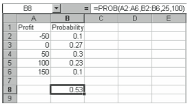
If you have a set of values and a set of probabilities associated with these values, you can find the probability that values in the range fall between two limits using the PROB function. The PROB function uses the following syntax:
=PROB(x range,probability range,lower limit,upper limit)
For example, the worksheet shown in Figure 4-12 shows the probability distribution for your company’s projected profits (in $1,000s) for the coming year, you can use the PROB function to find the probability that you make between $25,000 and $100,000 by entering the function as follows:
=PROB(A2:A6,B2:B6,25,100)
Rank and Percentile
Excel includes six functions used for finding rank and percentile on values in a data set.
LARGE
Use the LARGE function to find the kth largest value in a data set. While you can use the maximum function to find the largest value in a data set, you can use the LARGE function to find the runner up or third-place value. The LARGE function uses the following syntax:
=LARGE(data set range,k)
SMALL
Use the SMALL function to find the kth smallest value in a data set. Although you can use the MIN function to find the smallest value in a data set, you can use the SMALL function to find multiple values at the bottom. The SMALL function uses the following syntax:
=SMALL(data set range,k)
RANK
To find the rank of a value in a data set relative to other values in the data set, you can use the RANK function. The RANK function uses the following syntax:
=RANK(number,data set,order)
where number is the number whose rank you want to find, data set is the list of values against which you want to rank it, and order tells Excel to rank in ascending or descending order. Enter a nonzero value to rank the numbers in ascending order. Enter zero or leave the order parameter blank to rank in descending order.
PERCENTRANK
To find the rank of a value in a data set as a percentage, you can use the PERCENTRANK function. The PERCENTRANK function uses the following syntax:
=PERCENTRANK(data set,x,significance)
where x is the value whose rank you want to find, data set is the list of values against which you want to rank it, and significance tells Excel the number of significant digits it should use for the value. The value you get is between 0 and 1; you need to multiply by 100 to get the actual percent ranking.
PERCENTILE
Percentile is a measure that locates where a value stands in a data set. The kth percentile divides the data so that at least p percent are of this value or less and (100-p) percent are this value or more. If you have a set of data and need to find the value at a certain percentile, you use the PERCENTILE function in Excel. The PERCENTILE function uses the following syntax:
=PERCENTILE(data set range,k)
For example, if a score needs to be above the 80th percentile for admission, you can find which value defines that percentile by entering 0.8 for k.M
QUARTILE
The QUARTILE function in Excel is closely related to the PERCENTILE function. People often use quartiles, which order the values in a data set into quarters, when dividing populations into groups based on sales and survey data. The first quartile is the 25th percentile. The second quartile is the median, or 50th percentile. The third quartile is the 75th percentile. The fourth quarter is the maximum value. The QUARTILE function uses the following syntax:
=QUARTILE(data set range,quartile)
For the quartile parameter, enter 0 for the minimum value, 1 for the first quartile, 2 for the second quartile, 3 for the third quartile, or 4 for the maximum value.
Skewness (SKEW)
Like kurtosis, skewness is used to help determine the shape of a distribution. Skewness shows whether a distribution is symmetrical or not. A symmetric distribution, such as the normal curve, has a skew of zero. A positive skewness value indicates a long tail in the positive direction. A negative skewness value indicates a long tail in the negative direction. To find the skewness of a data set, enter the data set range as the single parameter in Excel’s SKEW function:
=SKEW(data set range)
Standard Normal Probability Distribution
Traditionally, to find the standard normal probability distribution, you must convert the normal random variable x to the standard normal distribution using the z-value formula, and then find the area under the standard normal distribution function below z. The normal probability distribution functions described earlier in this chapter shortens this process.
The Standard Normal Probability Distribution has a mean of 0 and a standard deviation of 1.
NORMSDIST
If you already have a z value, or if you’ve used the z-value formula STANDARDIZE described below to find a z-value, you can use the NORMSDIST function to find the probability that a random variable x is below z standard deviations from the mean. The NORMSDIST function uses the following syntax:
=NORMSDIST(z-value)
For example, if you create furniture that needs to fit people of various heights and know that the average American adult is 5’8″ tall, and the heights are normally distributed around this mean with a standard deviation of 4″, you can find the probability that one of your customers is less than 6’2″.
To use this function, you must first convert the data to the standard normal distribution as described below under “STANDARDIZE.” Doing so returns a z value of 1.5, meaning that 6’2″ is 1.5 standard deviations above the mean. When you enter 1.5 as the z-value parameter of the NORMSDIST function, the function returns the value 0.9331.
If you want to find the probability that a person is greater than 6’2″ tall, you just subtract this value from 1. If you want to find the probability that a person is between 5’4″ and 6′, you must make a few calculations. The probability that a person is less than 6′ tall is 0.8413. This means that the probability that a person is between the mean (5’8″) and 6′ is .3413 (because the probability that a person is less than 5’8″ is 0.5). Likewise, the probability that a person is between 5’4″ and 5’8″ is .34134474. Add these together to get 0.6826.
NORMSINV
If instead of having a value and needing to find the probability that a random variable falls below it, you know the probability for the range into which a random variable must fall and need to find the value defining this range, you can use the NORMSINV function.
To use the NORMSINV function, just enter the probability (between 0 and 1, of course) and the function returns the z-value below which the probability area you entered falls. If you choose a probability less than 0.5, the function returns a negative z-value. If you enter a probability greater than 0.5, the function returns a positive z-value. The NORMSINV function uses the following syntax:
=NORMSINV(probability)
STANDARDIZE
Traditionally, to answer probability questions about a normal distribution, you first convert the distribution to the standard normal distribution. The standard normal distribution has a mean of zero and a standard deviation of 1. To convert to the standard normal distribution, you find a z value using the STANDARDIZE function in Excel. The STANDARDIZE function uses the following syntax:
=STANDARDIZE(x,mean,standard deviation)
For example, if you have a product that costs an average of $6,000 to produce and a standard deviation of $800, what percentage of the items should you expect to cost more than $6,600?
To find out, enter the function as follows:
=STANDARDIZE(6600,6000,800)
The function returns the value .75. You can then use the NORMSDIST function to find the probability or area under the curve between 0 and .75.
The z-value tells you how far (in terms of the number of standard deviations) an individual observation is from the mean. It therefore also allows you to determine whether an observation is an outlier (unusually large or small) and therefore suspect. Z-values of less than –3 or greater than +3 are generally treated as outliers and call for closer inspection.
Sum of Squares of Deviations from Mean (DEVSQ)
To sum the squares of the deviations of the data points in a sample from the mean, you use the DEVSQ function. The DEVSQ function uses the following syntax:
=DEVSQ(data set range)
Standard Deviation
Standard deviation is a common measure of describing the spread of observations in a distribution. The standard deviation is equal to the square root of the variance.
STDEV
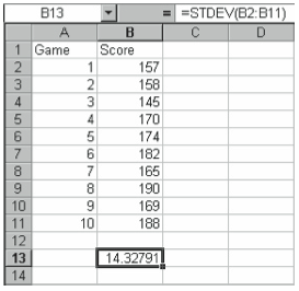
To find the standard deviation of a sample, ignoring logical values and text, use the STDEV function. This function has the following syntax:
=STDEV(data set range)
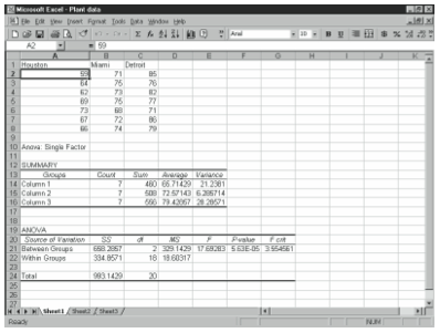
For example, to find the standard deviation in the worksheet containing a 10-game sample of a bowler’s scores, as shown in Figure 4-13, enter:
=STDEV(B2:B:11)
STDEVA
To find the standard deviation of a sample, and include cells containing the logical value TRUE as 1 and cells containing text or the logical value FALSE as 0 (zero), use the STDEVA function. This function has the following syntax:
=STDEVA(data set range)
STDEVP
To find the standard deviation of a population, ignoring logical values and text, use the STDEVP function. This function has the following syntax:
=STDEVP(data set range)
STDEVPA
To find the standard deviation of a population, and include cells containing the logical value TRUE as 1 and cells containing text or the logical value FALSE as 0 (zero), use the STDEVPA function. This function has the following syntax:
=STDEVPA(data set range)
t Distribution
If you’re working with a small sample (less than about 30 or 40), you can use the Student’s t-test instead of the z-value or z-score to find the probability with which a value falls below a certain number or to test how far an individual observation is from the mean. To do so, you use the TINV function.
TDIST
You can use the TDIST function to make inferences about the value of a population mean. For example, if you randomly select 20 people from a factory floor, ask them to try a new production method, and then find that they can produce 17.25 units an hour with a sample standard deviation of 3.3, you can find the probability that the population mean takes the value of 16 or less. To do so, you use Excel’s TDIST function. The function uses the following syntax:
=TDIST(x,degrees of freedom,tails)
For this example, the function takes the following form:
=TDIST(16,19,1)
Depending on your level of significance, you accept or reject the hypothesis.
The hypothesis in this example is one-tailed; that is, you’re interested in finding probabilities of values less than 16. If instead you need to find the probabilities of values both above and below x, your hypothesis is two-tailed.
TINV
If you know the probability and want to find the t-value, use the TINV function. This function has the following syntax:
=TINV(probability,degrees of freedom)
If this is based on a one-tailed t distribution, multiply the probability by 2.
TTEST
To find the probability associated with a Student’s t-test, use the TTEST function. The t-test is most frequently used to test for a difference between two means. The TTEST function uses the following syntax:
=TTEST(data set 1,data set 2,tails,type)
where type equals 1 for paired, 2 for two samples with equal variance, or 3 for 2 samples with unequal variance.
Trimming to the Mean (TRIMMEAN)
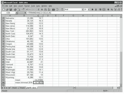
You calculate a trimmed mean by discarding a certain percentage of the lowest and the highest values from a data set to remove outliers, and then computing the mean of the remaining values. For example, a mean trimmed 50% is computed by discarding the lowest and highest 25% of the values and taking the mean of the remaining 50% in the middle. The TRIMMEAN function uses the following syntax:
=TRIMMEAN(data set range,percent)
where percent is entered as a decimal. For example, the spreadsheet of birth rates in the United States in Figure 4-14 shows the mean and a mean trimmed 25%.
Variance
Excel provides four functions for calculating variance, a measure of the variability between data values in a set. Variance is based on the difference between each value and the mean.
VAR
If the data set you’re working with is a sample and you do not want to include logical values or text from the set in the calculation, you use the VAR function. For example, if you’re using a new production process that is supposed to increase productivity and have a series of data for the numbers of parts produced each day, you can find the sample variance. The VAR function uses the following syntax:
=VAR(data set range)
VARA
If the data set is a sample but you want to include logical values or text in the calculation, you use the VARA function. Excel counts cells containing the logical value TRUE as 1 and cells containing text or FALSE 0. The VARA function uses the following syntax:
=VARA(data set range)
VARP
If the data set you’re working with is a population and you do not want to include logical values or text from the set in the calculation, you use the VARP function. The VARP function uses the following syntax:
=VARP(data set range)
VARPA
If the data set is a population but you want to include logical values or text in the calculation, you use the VARPA function. The VARPA function uses the following syntax:
=VARPA(data set range)
Weibull Distribution (WEIBULL)
The Weibull distribution is a skewed distribution commonly used to show product lifetimes, analysis of systems involving a “weakest link,” and wind speed.
The WEIBULL function uses the following syntax:
=WEIBULL(x,alpha,beta,cumulative)
where x is the value at which to evaluate the function, alpha and beta are parameters to the distribution, and cumulative specifies whether you want Excel to return the value of the function at exactly x (in which case you enter FALSE) or up to and including x (in which case you enter TRUE).
Z-Test (ZTEST)
Use the ZTEST function to find the two-tailed p-value of a z-test. The z-test standardizes x with respect to the data set, and returns the two-tailed probability for the normal distribution. You can use this function to determine the likelihood that a particular observation comes from a certain population.
The ZTEST function uses the following syntax:
=ZTEST(data set range,x,sigma)
If you don’t know the population standard deviation sigma (s), leave this parameter blank and Excel uses the sample standard deviation from the data set.
Leave a Reply