PivotTables got their name because you can easily rearrange, or “pivot,” them. For example, you can move row headings to become column headings, or vice versa, or you can change the hierarchy of fields within a row or column heading. You can also separate PivotTable data among pages.
Pivoting
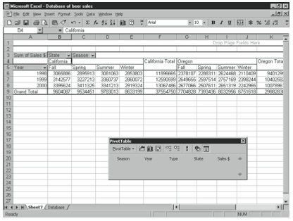
To pivot a PivotTable, just drag a heading to a different axis. For example, you can drag the Season field to the column heading to create a long, narrow table, as shown in Figure 8-7. By doing this, each state has its own subtable within the table.
You can also reorganize a PivotTable by changing the hierarchy of fields in a heading. For example, if you look back at the PivotTable in Figure 8-6, sales are grouped first by year and then by season within each year. However, if you drag the Season field to the left of the Year field, you can group first by season, and then within each season, by year.
Filtering Items in a Field
You can tell Excel which items you want to include in a PivotTable for each field. For ex- ample, if you don’t want to worry about sales in California for the moment, you can exclude California from the table. To do so, click the down arrow on the right side of the State heading and clear the California check box. Then click OK.
Separating Data Between Pages
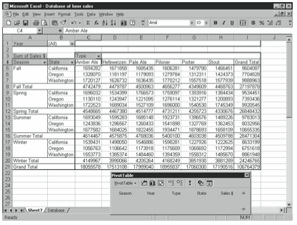
If your database is so large that your PivotTable is too long or wide to easily read without scrolling back and forth, you might want to view only certain parts of the data on a single worksheet page. For example, in the microbrewery database, you might want to put sales data for each year on a separate page. To do so, drag the Year field to the box labeled Drop Page Fields Here. You can view data for other years by clicking the down arrow on the right side of the Year heading and selecting a different year. You can also click the PivotTable button on the PivotTable toolbar and choose Show Pages from the pop-up menu to create new sheets in the workbook for each page field. Just select the page field from the list in the Show Pages dialog box, and click OK. Figure 8-8 shows how the PivotTable looks with Year as a page field, Type as a column heading, and Season and State as row headings.
Grouping PivotTable Data
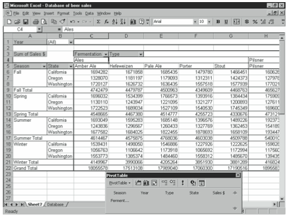
With some fields, you can create subgroups. For example, you may want to group the Types shown in Figure 8-8 into ales and lagers or dark beers and light beers. To create a group for the ales and another for the lagers, select all the types you want to include in the group. (You can select nonadjacent items by holding down the Ctrl key as you click.) Then choose the Data menu’s Group And Outline command and choose the submenu’s Group command. Excel names the groups Group1, Group2, and so forth. You can rename the groups to some- thing more descriptive by selecting the heading and typing a new name. Excel names the new field according to the field from which you’re creating the Groups. In this example, Excel names the new groups of fields Type2 because the Type field was grouped. You can change the name of the group field by selecting a group name and clicking the Field Settings but- ton on the PivotTable toolbar. Figure 8-9 shows how the PivotTable looks after grouping the types into Ales and Lagers and naming the group field Fermentation.
Leave a Reply