Excel supplies many helpful commands that make creating and editing your workbooks easier and more efficient. If you anticipate spending any time at all working with Excel, it makes good sense for you to learn how these tools work and when they come in handy.
Erasing Cell Contents
You can erase the contents and formatting from a single cell or a range quickly and easily. To erase, follow these steps:
- Select the cell or range you want to clear.
You can select a cell by clicking it. You can select a range of cells by dragging the mouse from one corner of the range to the opposite corner of the range. - Delete the cell contents.
Press the Delete key to erase all contents and formatting, or choose the Edit menu’s Clear command to specify what you want to erase. Choose one of the four commands from the submenu, as shown in Table 2-3.ALL ERASES ALL CONTENTS AND FORMATTING Formats Erases formatting but leaves contents. Contents Erases the contents but leaves the formatting. Comments Erases any comments inserted using the Insert menu’s Comment command. Table 2-3. The Clear submenu’s commands.
Undoing Mistakes
If you make a mistake while entering data or editing your worksheet, you can use the Undo toolbar button to reverse the effects of your last actions. You can also undo the Undo operation by clicking the Redo toolbar button. To reverse the effects of a series of most recent actions, click the arrow beside the Undo toolbar button and select multiple actions from the list. To redo a series of last actions, click the arrow beside the Redo toolbar button and select multiple actions from the list.
Copying, Cutting, and Pasting
You can copy or cut the contents of cells and ranges and then paste them into other locations. This means you don’t have to repeatedly type a label, value, or formula. You can type the entry just once and then copy or move it.
Copying Labels and Values
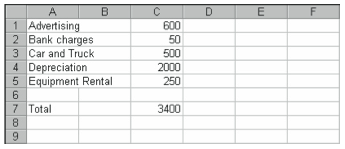
Suppose, for example, that the numbers shown in column C of the budgeting worksheet represent the budgeted expenses for January and that the same figures are projected for February and March (see Figure 2-13). Rather than reenter the same values, you could copy the values already stored in column C.
To copy the labels and values for such an operation, follow these steps:
- Select the cell or range to be copied.
In Figure 2-13, this would mean you select the range C1:C5. The easiest method for selecting a specific cell or range is by clicking or clicking and dragging the mouse. - Click the Copy toolbar button, or choose the Edit menu’s Copy command.
When you do this, Excel places a copy of the labels and values on the clipboard. - Select the destination cell or the cell in the upper left corner of the destination range.
If you want to duplicate the selected cells more than once, select the multiple destination ranges in their entirety. For the worksheet shown in Figure 2-13, for example, you would select the range D1:E5. - Click the Paste toolbar button, or choose the Edit menu’s Paste command.
When you do this, Excel copies the worksheet range from the clipboard into the specified worksheet range (see Figure 2-14).
Figure 2-14. A worksheet with two copies of C1:C5 pasted in D1:E5.
Copying Formulas
When you copy labels and values, Excel duplicates the contents of the copied cell or cells and pastes the data into the selected range. When you copy a formula, however, Excel adjusts any cell references used in the formula. This important difference can be illustrated by copying the formula in cell C7 of Figure 2-14, =C1+C2+C3+C4+C5, into cells D7 and E7. To do this, follow these steps:
- Select the cell or range with the formula(s) you want to copy.
In the example of the worksheet shown in Figure 2-14, you would select cell C7. - Click the Copy toolbar button.
Excel moves a copy of the formula in cell C7 to the clipboard. - Select the destination range D7:E7.
In the example of the worksheet shown in Figure 2-14, you would select the range D7:E7. - Click the Paste toolbar button.
Excel adjusts the formulas for the column in question and pastes the formula =D1+D2+D3+D4+D5 into cell D7 and the formula =E1+E2+E3+E4+E5 into cell E7. Figure 2-15 shows the worksheet after copying the formula.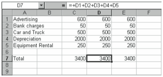
Figure 2-15. The budgeting worksheet after copying the formula in cell C7 into cells D7 and E7.
The formula changes that Excel makes aren’t a mistake. Excel assumes—unless you tell it otherwise—that the cell references in your formulas are relative. When Excel copies and pastes a formula with relative cell references, it adjusts them.
To prevent Excel from automatically adjusting the relative references of copied formulas, you can make them absolute. Simply place a dollar sign ($) in front of the part or parts you don’t want Excel to adjust. For example, to tell Excel not to adjust the formula at all, place a dollar sign in front of both the column letter and row number like this $A$1. To allow Excel to adjust row numbers but not column letters, put a dollar sign in front of the column letter but not the row number, like this: $A1. And to allow Excel to adjust column letters but not row numbers, put a dollar sign in front of the row number but not the column letter, like this: A$1.
Special Pasting Options
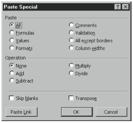
If you want to specify pasting options, instead of just clicking the Paste button after copying or cutting, choose the Edit menu’s Paste Special command. Excel displays the Paste Special dialog box shown in Figure 2-16. To paste a row of cells as a column of cells or vice versa, select the Transpose check box. To paste only a portion of the copied or cut cells’ contents, click a Paste option button other than All. For example, to paste only the comments in a cell, click the Comments option button under Paste. To add, subtract, multiply, or divide the values in the copied range with the values in the destination range, click the Add, Subtract, Multiply, or Divide option button under Operation. To tell Excel it shouldn’t paste blank cells over values, select the Skip Blanks check box.
Moving Labels, Values, and Formulas
To move, rather than copy, a selected range, follow the same procedure, but click the Cut toolbar button or choose the Edit menu’s Cut command instead of choosing the Copy command. Excel removes the selected contents from their original location and allows you to paste them in a new location.
You can also move a cell or range with the mouse by selecting the cell or range and pointing to the black border around the cell or range so that the mouse pointer changes from a cross to an arrow. Then drag the cell or range to a new location.
Filling Ranges
To continue a pattern you’ve begun, use the fill handle in the lower right corner of a cell or range. For example, if you begin the pattern 0, 5, 10 and want to continue it down a column, select the cells holding these values and click the little black square in the lower right corner of the range. The mouse pointer changes from a white outlined cross to a black cross. Now drag the mouse down the column as far as you want the pattern to go. This procedure also works for easily identifiable patterns of labels, such as months of the year and days of the week.
Inserting and Deleting Cells, Rows, Columns, and Worksheets
Excel lets you insert and delete cells, rows, columns, and worksheets in your workbook with speed and efficiency. You can easily delete what you no longer need or insert new items between existing entries when you need more space.
Using the Insert Command
To insert a row, click any cell in the row below where you want a row inserted. Then choose the Insert menu’s Rows command.
To insert a column, click any cell in the column to the right of where you want a column inserted and choose the Insert menu’s Columns command.
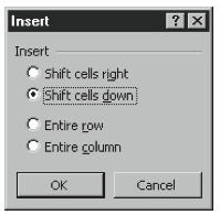
To insert a cell in a column or row, choose the Insert menu’s Cells command. Excel displays the Insert dialog box shown in Figure 2-17. Click the Shift Cells Right button to insert a new cell in a row or click the Shift Cells Down button to insert a new cell in a column. After you’ve selected the appropriate option button, click OK.
To insert a worksheet, display the worksheet in front of which you want to create a new worksheet and choose the Insert menu’s Worksheet command.
Using the Delete CommandM
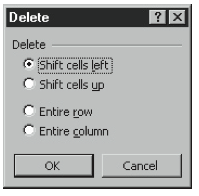
To delete a cell, range, row, or column, select the specific cell or range or any cell in the row or column you want to delete and choose the Edit menu’s Delete command. Excel displays the Delete dialog box shown in Figure 2-18. Describe whether you want to shift the remaining cells up or to the left, or whether you want to delete the entire row or column, and click OK.
Excel attempts to adjust the cell references and range definitions used in formulas for row and column insertions and deletions. For example, if a formula uses values in column C and you delete column B so that column C becomes the new column B, Excel adjust the formulas to read column B. If you delete a cell referenced in a formula, however, Excel replaces the formula’s reference with the error message #REF, indicating that the formula originally referenced a now-deleted cell.
Using Find and Replace
Excel provides two commands that you can use to search your workbook for specific entries. The Find command simply locates the contents you’re looking for. The Replace command locates the contents and then gives you the option of replacing them with a new label, value, or formula.
Using the Find Command
To search your worksheet and locate specific entries, choose the Edit menu’s Find command. Excel displays the Find dialog box shown in Figure 2-19.
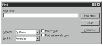
Enter the label, value, or formula you want to find in the Find What text box, use the drop-down list boxes and check boxes to specify the parameters of your search, and then click Find Next to begin. If Excel finds an entry that matches your search parameters, it moves the cell selector to that cell. To resume searching, click Find Next again. Click Close when you’re finished.
Using the Replace Command
When you choose the Edit menu’s Replace command, Excel displays the Replace dialog box shown in Figure 2-20.
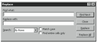
Enter the item you want to find in the Find What text box and the label, value, or formula with which you want to replace it in the Replace With text box. Use the drop-down list box and check boxes to specify the parameters of your search.
Click Find Next and Replace to search for and replace entries one by one. Or click Replace All to have Excel automatically find and replace all occurrences of the entry without requesting verification from you. Click Close when you’re finished.
Checking Your Spelling
Excel lets you check the spelling of a selected word, within a selected range or within an entire workbook. To check spelling, click the Spelling toolbar button. If Excel finds a word that’s not in its dictionary, it displays the Spelling dialog box (see Figure 2-21).
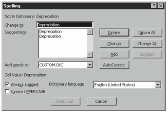
If one of Excel’s suggestions is correct, select it from the list box and click Change. If you want to change all occurrences of the misspelling to the suggestion you selected, click Change All. If you want to ignore the misspelling and continue, click Ignore. If you want to Ignore all occurrences of the spelling, click Ignore All. If you want Excel to recognize the word in future documents and spell checks, you can add it to the dictionary by clicking Add.
Leave a Reply