With proper formatting, your worksheets are easier to read and more visually attractive. Fortunately, Excel includes a rich set of easy-to-use tools for formatting your workbook data so it’s more enjoyable and easier to read.
Using a Predesigned Format
Excel’s AutoFormat feature performs many standard formatting tasks in a single operation: setting fonts, aligning labels, setting column width and row height, establishing numeric and date/time formats, and adding borders and rules.
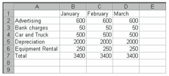
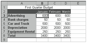
To use AutoFormat, you first enter worksheet labels, values, and formulas, as shown in Figure 2-22.
To use the AutoFormat command, follow these steps:
- Select the worksheet range you want to format.
In Figure 2-22, you would select the range A1:D7. - Choose the Format menu’s AutoFormat command.
Excel displays the AutoFormat dialog box (see Figure 2-23).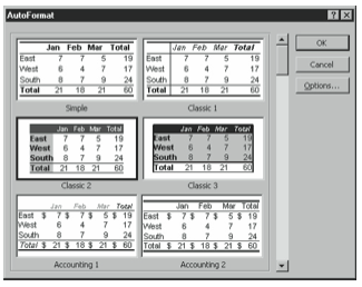
Figure 2-23. The AutoFormat dialog box. - Select the AutoFormatting options you want to use.
Click the Options button if you want to specify which AutoFormatting options should be applied to your worksheet selection. When you do this, Excel adds Options check boxes to the AutoFormat dialog box. Select and clear these check boxes to selectively apply individual components of an AutoFormat. - Select an AutoFormat by clicking it.
The AutoFormat pictures show roughly what the AutoFormat formatting looks like. - Click OK to apply the format to the range you selected.
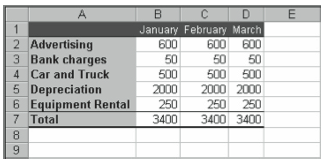
Figure 2-24 shows what the budgeting worksheet looks like after the AutoFormat selected in Figure 2-23 is applied.
Formatting Manually
As you create more complex and specialized worksheets, your formatting efforts require similar treatment. The following paragraphs briefly detail each of Excel’s formatting features.
Aligning Labels and Values
Excel normally aligns numbers against the right edge of a cell and text against the left edge. You can override these default alignments by using the Left Align, Center, Right Align, and Merge And Center buttons on the toolbar.
The Left Align, Center, and Right Align toolbar buttons work as you might expect. For example, to left align the contents of selected cells, click the Left Align button.
The Merge And Center toolbar button is a little more complex. It lets you center a label across a selection of cells. For example, you can insert a new row and enter a label in cell A1 of the budgeting worksheet (as shown in Figure 2-25) and then center it across the range A1:D1.
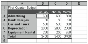
To center the label,first select the range and then click the Merge And Center toolbar button. Figure 2-26 shows the worksheet after this alignment.
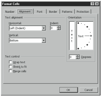
You can access a more sophisticated array of alignment features by selecting the cell or range you want to align, choosing the Format menu’s Cells command, and clicking the Alignment tab in the Format Cells dialog box (see Figure 2-27). The Horizontal drop-down list box lets you align cell contents in the same ways as the Left Align, Center, Right Align, and Merge And Center tools do. The Vertical drop-down list box allows you to align cell contents at the top, center, or bottom of the cell. The Orientation box allows you to rotate the cell contents.
The Text Control boxes provide you with several more specialized alignment options. The Wrap Text check box allows you to wrap a long line of text into multiple lines in a single cell. The number of lines varies depending on the amount of text and the width of the cell. The Shrink To Fit check box allows you to decrease the size of the numbers or letters in a cell so that they fit in the current size constraints of the cell. The Merge Cells check box allows you to combine cells into larger, single cells.
Formatting Numbers
You can assign numeric formats such as dollar signs, percentage symbols, and commas. To quickly assign these specific common formats, select the cell or range you want to format and click the Currency Style, Percent Style, or Comma Style toolbar button. To assign other numeric formats, follow these steps:
- Choose the Format menu’s Cells command, and click the Number tab.
Excel displays the Number tab of the Format Cells dialog box, as shown in Figure 2-28.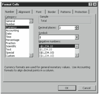
Figure 2-28. The Number tab of the Format Cells dialog box. - Select a numeric formatting category from the list on the left.
In a budgeting worksheet, you would probably choose the Accounting category. - Use the boxes and buttons for the category you chose to specify the exact formatting.
In a budgeting worksheet, for example, you might need to select a different currency symbol from the Symbol drop-down list box. - Click OK.
Changing Font and Font Size
Excel offers a wide variety of choices for changing a selected font’s appearance, such as by adding boldfacing or underlining, for changing a font, and for specifying a different size.
To add effects such as boldfacing, italics, and underlining, you can use the Bold, Italic, and Underline font buttons on Excel’s toolbar. To use any of these buttons, simply select the worksheet range you want to format and then click the button.
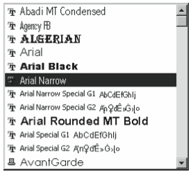
To change the font of text, click the down arrow beside the Font toolbar button and select a font from the list. If you open the Font drop-down list box, Excel displays the font’s name using the font itself, so you can preview what the font looks like (see Figure 2-29). Fonts listed with a TT icon beside them are TrueType fonts. Fonts built into your printer have a printer icon next to them. If you use a TrueType font, the font you see on your screen will be the same one that the printer prints. If you use a scalable printer font and the printer you use doesn’t support your selection, the printer uses the closest-matching font.
To change the size of text, click the down arrow beside the Size toolbar button. Fonts are measured using points. One point is 1/72 of an inch. So a point size of 18 means that the font is 1/4 inch tall. Excel’s default point size is 10. You probably don’t want to use fonts smaller than 10 points for legibility.
Adding Color to Cells and Text
Excel allows you to add color and shading to your data to help you organize, clarify, and emphasize the information on your worksheet—as well as to add interest.
To change the color of text, select the range you want to color, click the down arrow beside the Font Color toolbar button, and then select a color for the text.
To add a background color to a range of cells, select the range, click the down arrow beside the Fill Color toolbar button, and select a color for the cell background.
Creating Borders
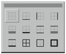
To polish your worksheets and make them easy to read, you can add borders with the Borders toolbar button. To add a border to a cell or range, select the cell or range and click the down arrow beside the Borders toolbar button.
Excel displays the box shown in Figure 2-30, illustrating common border patterns and placements. To select a design for your cell or range, click it.
Modifying Column and Row Size
As you reformat the labels and values in your worksheet, you may need to modify the standard column and row sizes to accommodate your formatting changes. To quickly increase the column width to accommodate all text in the column but include no extra white space, double-click the right border of that column heading. Normally, Excel automatically increases row height when you increase point size, but you can perform the same trick on rows by double-clicking the lower border of a row heading. This expands the row to the smallest height possible that still fits all entries within that row.
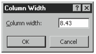
To specify exact column width, select any cell in that column, choose the Format menu’s Column command, and choose the Column submenu’s Width command. Enter the width in characters in the Column Width text box (see Figure 2-31), and click OK.
To specify exact row height, select any cell in that row and choose the Format menu’s Row command and then choose the Row submenu’s Height command. Enter the height in points in the Row Height text box, and click OK. To hide a row, select any cell in the row and choose the Format menu’s Row command and then choose the Row submenu’s Hide command. To redisplay a hidden row, select a range that includes cells in the rows above and below the hidden row. Then choose the Format menu’s Row command, and choose the Row submenu’s Unhide command.
To hide a column, select any cell in the column and choose the Format menu’s Column command and then choose the Column submenu’s Hide command. To redisplay a hidden column, select a range that includes cells in the columns to the left and right of the hidden column. Then choose the Format menu’s Column command, and choose the Column submenu’s Unhide command.
Using the Format Painter
Excel provides a feature that allows you to quickly copy the formatting from one cell to another while leaving the cell’s contents intact. To copy cell formatting, select the cell with the formatting you want to copy. Next, click the Format Painter toolbar button, and then select the cell or range to which you want to apply the formatting.
Conditional Formatting
If you want to format only those cells that meet certain criteria, you can use Excel’s Conditional Formatting feature. You might want to do this, for example, if you want to highlight cells in a budgeting worksheet that contain values larger than 200.
To apply conditional formatting, select the range of cells you want to include in the conditional formatting filters and then follow these steps:
- Choose the Format menu’s Conditional Formatting command.
Excel displays the Conditional Formatting dialog box (see Figure 2-32).
Figure 2-32. The Conditional Formatting dialog box. - Enter the first criteria, using the drop-down list boxes and text boxes provided.
For example, if you want Excel to display values greater than $500 in red italic boldface, indicate that you want to conditionally format cells with values greater than 500, as shown in Figure 2-32. - Click Format to describe how you want Excel to format the cells with contents that fit your criteria.
When you do this, Excel displays a variant of the Format Cells dialog box. Use it specify the font, font size, font effects, and font color you want to use for cells that contain labels or values meeting your conditions. Click OK to close the Format Cells dialog box and return to the Conditional Formatting dialog box. - Add the conditional formatting rule.
Click Add, and Excel adds the conditional formatting rule. If you want to specify multiple criteria, repeat steps 1 and 2 for the other criteria. - Click OK.
Excel applies the conditional formatting, as shown in Figure 2-33. The budgeting worksheet displays values greater than 500 highlighted in red italic boldface.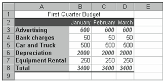
Figure 2-33. Conditional formatting applied to values.
Leave a Reply