Excel’s power stems from its ability to perform calculations on the values you’ve stored in a workbook—something you do with formulas and functions. This section describes how to construct formulas; use Excel’s predefined formulas, called functions; and use range names in formulas. It also shows how to open saved workbooks.
Entering Formulas
Excel calculates formulas automatically. You enter them in a worksheet cell in the same way as you do with labels and values. In the cell, however, Excel displays not the formula, but its result. For example, if you enter a formula that says to add 4 and 2, Excel retains the formula and displays it in the formula bar when the cell is selected, but Excel displays the result, 6, in the worksheet itself.
Formula Fundamentals
Formulas must begin with the equal sign (=); that’s how Excel distinguishes them from values and labels. You can construct formulas that subtract, multiply, divide, and exponentiate. The – symbol means subtraction, the * means multiplication, the / means division, and the ^ means exponential operation. Table 2-1 shows the different mathematical operators and the results they return.
| FORMULA ENTERED | RESULT DISPLAYED IN CELL |
| =4+2 | 6 |
| =4-2 | 2 |
| =4*2 | 8 |
| =4/2 | 2 |
| =4^2 | 16 |
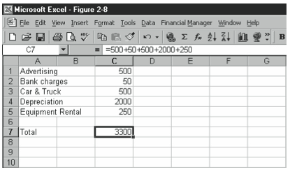
Figure 2-8 shows a simple budgeting worksheet built from Figure 2-5. The formula used in cell C7 appears in the formula bar and the result is displayed in the worksheet.
To build more complicated formulas, you need to recognize the standard rules of operator precedence: Excel first performs exponential operations, then multiplication and division operations, and finally, addition and subtraction.
For example, in the equation =1+2*3^4, Excel first raises 3 to the fourth power to get 81. It then multiplies this value by 2 to get 162. Finally, it adds 1 to this value to get 163.
To override these rules, you must use parentheses. You can use multiple sets of parentheses in a formula as need be. Excel first performs the function in the innermost set of parentheses. Look at the following formulas in Table 2-2 as an example.
| FORMULA ENTERED | RESULT DISPLAYED IN CELL |
| =1+2*3^4 | 163 |
| =(1+2)*3^4 | 243 |
| =((1+2)*3)^4 | 6561 |
Using Cell References
In the budgeting worksheet, you could total the budgeted expenses by entering the formula =500+50+500+2000+250 in cell C7. There is, however, a practical problem with this approach: You would need to rewrite the formula each time any of the values changed. Because this approach is unwieldy, Excel also allows you to use cell references in formulas. When a formula includes a cell reference, Excel uses the value that cell contains. For example, to add the budgeted amounts on your budgeting worksheet using a formula with cell references, follow these steps:
- Move the cell selector to C7.
You can do this by clicking cell C7. Or you can use the arrow keys. - Type =C1+C2+C3+C4+C5.
If you make a mistake entering this formula, you can edit it in the same way that you edit any label or value. - Press the Enter key, or click the Enter button.
Excel enters your formula in the cell, calculates the formula, and then displays the formula result (see Figure 2-9).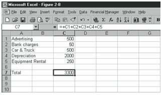
Figure 2-9. A worksheet with cell references used in a formula.
To reference a cell on the same worksheet as the formula, you need to supply only the column-letter-and-row-number cell reference. To reference cell C1 on the same worksheet, for example, you enter C1.
You can also reference cells on other worksheets. To reference a cell on another worksheet in the same workbook, however, you need to precede the cell reference with the name of the worksheet and an exclamation point symbol. To reference cell C1 on the worksheet named Sheet2, for example, you enter Sheet2!C1.
You can reference cells in other workbooks, too. To do this most easily, open the other workbooks, begin building your formula as described earlier in this chapter, and then click the other workbook cell you want to reference at the point you want to include the reference. Excel then writes the full cell reference for you, which includes the workbook name. An external reference to cell C1 on the worksheet named Sheet2 in the workbook named Budget might be written as =[Budget.xls]Sheet2!$C$1.
Understanding Worksheet Recalculation
As you build and edit your worksheet, Excel automatically updates the formulas and recalculates their results. For example, in the budgeting worksheet, if you change the value in cell C1 from 500 to 600, Excel recalculates any formulas that use the value stored in cell C1. As a result, the formula in cell C7 returns the value 3400—an increase of one hundred.
In simple worksheets, such as the one shown in Figure 2-9, recalculation takes place so quickly you won’t even be aware it’s occurring. In larger worksheets with hundreds or even thousands of formulas, however, recalculation is much slower. The mouse pointer changes to the hourglass symbol when Excel is busy recalculating.
If you don’t want Excel to automatically recalculate formulas as you’re working, choose the Tools menu’s Options command and click the Calculation tab. Then click the Manual option button under Calculation, and click OK. The word Calculate appears on the status bar when your worksheet needs to be recalculated. You can force recalculation by pressing the F9 key.
Formula Errors
It’s possible to build an illogical or unsolvable formula. When you do, Excel displays an error message in the cell rather than calculating the result. The error message, which begins with the # symbol, describes the error. Suppose, for example, that you enter the formula =1/0 in a cell. Because division by zero is an undefined mathematical operation, Excel can’t solve the formula. To alert you to this, Excel displays the error message #DIV/0!
Another common error is a circular reference. This occurs when two or more formulas indirectly depend on one another to achieve a result. For example, if the formula in cell A1 is =A2 and the formula in cell A2 is =A1+A3+A4, A1 depends on A2 and A2 depends on A1. Excel displays a warning and the Circular Reference toolbar when you create a circular reference. Excel identifies circular references by displaying the word Circular on the status bar and showing the address of the cell whose formula completed the “circle.” It also draws arrows between the cells causing the circle.
To fix a formula error, edit the erroneous formula using the same techniques as with label and value editing. Move the cell selector to the cell holding the formula, click the formula bar, and edit the formula. When the formula is correct, set it by moving the cell selector, pressing the Enter key, or clicking the Enter button.
Using Functions
Excel provides several hundred prebuilt formulas, called functions, that provide a shortcut to constructing complicated or lengthy formulas. In general, a function accepts input values, or arguments, then makes some calculation and returns a result.
Excel provides financial, statistical, mathematical, trigonometric, and even engineering functions. Each function has a name that describes its operation. The function that adds values is named SUM, for example, and the function that calculates an arithmetic mean, or average, is named AVERAGE.
Most functions require arguments, or input values, which you enclose in parentheses. The ROUND function, for example, rounds a specific value to a specified number of decimal places. To round the value 5.75 to the nearest tenth, you could use the function shown below:
=ROUND(5.75, 1)
Even if a function doesn’t require arguments, you still need to include the parentheses. For example, the function PI returns the mathematical constant Pi. The function needs no arguments, but you still need to enter it as =PI().
Functions can use values, formulas, and even other functions as arguments. If entered in the budgeting worksheet shown in Figure 2-9, for example, each of the following functions returns the same result, 3300:
=SUM(C1:C5)
=SUM(C1,C2,C3,C4,C5)
=SUM(500,50,500,2000,250)
=SUM(SUM(C1),SUM(C2),SUM(C3),SUM(C4),SUM(C5))
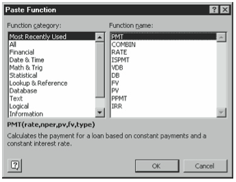
To most easily insert complicated functions and reduce your chance of error, click the Paste Function toolbar button or choose the Insert menu’s Function command. This displays the Paste Function dialog box shown in Figure 2-10. Select the function category from the list on the left and the specific function from the list on the right. Because some of the functions are a little difficult to recognize or distinguish by name, Excel describes what the selected function does at the bottom of the Paste Function dialog box. When you have found the function you want to use, click OK.
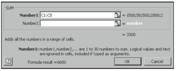
Excel displays the second Paste Function dialog box with text boxes you can use to identify or supply the arguments required for the function (see Figure 2-11). If necessary, drag this dialog box to another portion of your screen to see the cells you want to include in the function. To enter cell data in an argument text box, click that box and then select the cell or range of cells in your worksheet that goes in the box. Excel highlights the cell or cells you selected with a flashing box. To enter cell data in another argument text box, click that box and select the cell or range in your worksheet that contains the data required for that box. Click OK when you’re finished. Excel pastes the function in the cell.
Naming Cells and Ranges
In a small sample worksheet such as the one shown in Figure 2-9, it’s not too difficult to remember that cell C1 contains the advertising expenses, C2 contains the bank charges, and so on. In the real world, however, Excel worksheets can be much more complex, and keeping track of what each cell represents becomes correspondingly more difficult. In this way, instead of referring to cell C1 in a formula, you could refer to Advertising if you first name the individual cell Advertising. For example, if you named cells C1, C2, C3, C4, and C5 Advertising, Bank, Car, Depreciation, and Equipment, respectively, the following two formulas would be identical:
=C1+C2+C3+C4+C5
=Advertising+Bank+Car+Depreciation+Equipment
To name a cell or range, follow these steps:
- Select the cell or range of cells to be named.
You can select a cell by clicking it or by using the arrow keys to move the cell selector to thecell.Youcanselectarangeofcellsbyclickingononecorneroftherangeandthen,while holding down the mouse button, dragging the mouse to the opposite corner of the range. - Choose the Insert menu’s Name command, and choose the Name submenu’s Define command.
Excel displays the Define Name dialog box (see Figure 2-12).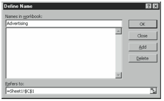
Figure 2-12. The Define Name dialog box. - Enter a name in the Names In Workbook text box.
Range names must begin with a letter, not a number. They cannot include spaces, and they shouldn’t look like cell references or function names. - Click Add.
To create another name, click Add and then repeat steps 1-3. To finish creating names, click OK.
Range names are useful in formulas and functions, but that’s not their only use. Once you name a range, you can use the name in place of the range definition whenever Excel asks you for a range. For example, if you use the Go To command, you could enter a name instead of a cell address.
Leave a Reply