The business planning starter workbook has seven parts: the inputs forecast, Balance Sheet, Common Size Balance Sheet, Income Statement, Common Size Income Statement, Cash Flow Statement, and Financial Ratios Table. I want to briefly describe the calculations that occur within each of these parts in case you have questions or in case you want to modify the starter workbook so it works for your situation.
Forecasting Inputs
The inputs area of the business planning starter workbook has one set of formulas. The second row identifies the period for which the results are calculated. The period identi- fier numbers the periods for which values are entered. The start of the first period is stored in cell B2 as the integer 0. Periods that follow are stored as the previous period plus 1.
The period identifiers in the Balance Sheet, Common Size Balance Sheet, Income State- ment, Cash Flow Statement, and Financial Ratios Table schedules use similar formulas.
Balance Sheet
The Balance Sheet schedule has 19 rows with calculated data and one row with the text label Period (see Figure 10-2). (As in the inputs area of the business planning starter workbook, the period identifier numbers the periods for which values are forecasted.) The rest of the Balance Sheet’s values are described in the paragraphs that follow.
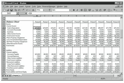
Cash & Equivalents
The Cash & Equivalents figures show the projected cash on hand at the end of each of the forecasting periods. The starting balance is the value you enter in the inputs area of the business planning starter workbook. The balance for the first and subsequent periods is pulled from the Cash Flow Statement schedule, where it is calculated.
Accounts Receivable
The Accounts Receivable (A/R) figures show the net receivables held as of the end of each forecasting period. The starting balance is the value you enter in the inputs planning area of the business starter worksheet. The balance for the first and subsequent periods is based on the Sales Revenue and the # Periods of Sales in A/R values you enter in the inputs area of the business planning starter workbook. For example, the formula for the first period is:
=C7*C31
The formula for the second period is:
=D7*D31
and so on.
Inventory
The Inventory values show the dollar total of the inventory held at the end of each fore- casting period. The starting balance is the value you enter in the inputs area of the busi- ness planning starter workbook. The balance for the first and subsequent periods is the previous period balance plus any inventory purchases or production costs minus any cost of sales. For example, the formula for the first period is:
=B45+C9-C32
The formula for the second period is:
=C45+D9-D32
and so on.
Other Current Assets
The Other Current Assets figures show the dollar total of the other current assets held at the end of each forecasting period. The starting balance for Other Current Assets is the value you enter in the inputs area of the business planning starter workbook. The balance for the first and subsequent periods is the previous balance plus the change in the balance. For example, the formula for the first period is:
=B46+C11
The formula for the second period is:
=C46+D11
and so on.
Total Current Assets
The Total Current Assets figures show the dollar total of the current assets at the end of each of the forecasting horizons. The balance at any time is the sum of Cash & Equivalents, Accounts Receivable, Inventory, and Other Current Assets. For example, the formula for the starting Total Current Assets balance is:
=SUM(B43:B46)
The formula for the second period is:
=SUM(C43:C46)
and so on.
Plant, Property, & Equipment
The Plant, Property, & Equipment figures show the original dollar cost of the plant, prop- erty, and equipment at the end of each forecasting horizon. The starting Plant, Property, & Equipment balance is the value you enter in the inputs area of the business planning starter workbook. The balance for the first and subsequent periods is the previous balance plus any additions to the plant, property, and equipment accounts. For example, the formula for the first period is:
=B48+C13
The formula for the second period is:
=C48+D13
and so on.
Less: Accumulated Depreciation
The Accumulated Depreciation figures show the cumulative depreciation expenses charged through the current period for the plant, property, and equipment. The starting balance is the value you enter in the inputs area of the business planning starter workbook. The bal- ance for the first and subsequent periods is the previous balance minus the current period’s changes in accumulated depreciation. For example, the formula for the first period is:
=B49-C15
The formula for the second period is:
=C49-D15
and so on. Because the accumulated depreciation is shown as a negative amount, you need to subtract the positive number pulled from the forecasting inputs.
Net Plant, Property, & Equipment
The Net Plant, Property, & Equipment figures show the difference between Plant, Prop- erty, & Equipment and Accumulated Depreciation at the end of each of the forecasting horizons. For example, the formula for the starting balance is:
=B48+B49
The formula for the first period is:
=C48+C49
and so on. Because the Accumulated Depreciation balance is shown as a negative amount, you simply add these two amounts in the formula for the Net Plant, Property, & Equip- ment amount.
Other Noncurrent Assets
The Other Noncurrent Assets figures show the dollar total of any other noncurrent assets held at the end of each of the forecasting periods. The starting balance is the value you enter in the inputs area of the business planning starter workbook. The balance for the first and subsequent periods is the previous period balance plus the change in the account in the current period. For example, the formula for the first period is:
=B51+C17
The formula for the second period is:
=C51+D17
and so on.
Total Assets
The Total Assets figures show the dollar total of all the assets held at the end of the fore- casting periods. The balance at any time is the sum of Current Assets; Net Plant, Property, & Equipment; and Other Noncurrent Assets. For example, the formula for the starting balance is:
=B47+B50+B51
The formula for the first period is:
=C47+C50+C51
and so on.
Accounts Payable
The Accounts Payable figures show the debt that is related to the cost of sales outstanding at the end of each forecasting period. The starting balance is the value you enter in the inputs area of the business planning starter workbook. The balance for the first and subsequent periods is Cost of Sales for the period times # of Periods of Cost of Sales in A/P. For ex- ample, the formula for the first period is:
=C19*C32
The formula for the second period is:
=D19*D32
and so on.
Accrued Expenses
The Accrued Expenses figures show the debt that is related to the operating expenses out- standing at the end of each forecasting period. The starting balance is the value you enter in the inputs area of the business planning starter workbook. The balance for the first and subsequent periods is the operating expenses times # of Periods Operating Expenses in A/E. For example, the formula for the first period is:
=C21*SUM(C33:C35)
The formula for the second period is:
=D21*SUM(D33:D35)
and so on.
Other Current Liabilities
The Other Current Liabilities figures show the dollar total of other debts outstanding at the end of the forecasting periods that will be paid within the current year or business cycle. The starting balance is the value you enter in the inputs area of the business planning starter workbook. The balance for the first and subsequent periods is the previous balance plus the change in the current period. For example, the formula for the first period is:
=B59+C23
The formula for the second period is:
=C59+D23
and so on.
Total Current Liabilities
The Total Current Liabilities figures show the dollar total of all the current liabilities at the end of each of the forecasting periods. The balance at any time is the sum of Accounts Payable, Accrued Expenses, and Other Current Liabilities. For example, the formula for the starting balance is:
=SUM(B57:B59)
The formula for the first period is:
=SUM(C57:C59)
and so on.
Long-Term Liabilities
The Long-Term Liabilities figures show the dollar total of the long-term outstanding debt at the end of each forecasting period. The starting balance is the value you enter in the inputs area of the business planning starter workbook. The balance for the first and subsequent periods is the previous balance plus any changes in the Long-Term Liabilities balance in the current period. For example, the formula for the first period is:
=B62+C25
The formula for the second period is:
=C62+D25
and so on.
Other Noncurrent Liabilities
The Other Noncurrent Liabilities figures show the dollar total of any other noncurrent outstanding debt at the end of each forecasting period. The starting balance is the value you enter in the inputs area of the business planning starter workbook. The balance for the first and subsequent periods is the previous period balance plus the change in the current pe- riod. For example, the formula for the first period is:
=B63+C27
The formula for the second period is:
=C63+D27
and so on.
Total Noncurrent Liabilities
The Total Noncurrent Liabilities figures show the dollar totals of the long-term debt and the other noncurrent outstanding debt at the end of each of the forecasting periods. The balance at any time is the sum of Long-Term Liabilities and Other Noncurrent Liabilities. For example, the formula for the starting balance is:
=B62+B63
The formula for the first period is:
=C62+C63
and so on.
Owner Equity
The Owner Equity figures show the dollar totals of the owner equity accounts at the end of each forecasting period. The starting balance is the value you enter in the inputs area of the business planning starter workbook. The balance for the first and subsequent periods is the previous period balance plus Net Income After Taxes for the period plus other ad- justments, such as additional capital contributions and dividends. For example, the formula for the first period is:
=B65+C29+C116
The formula for the second period is:
=C65+D29+D116
and so on.
Total Liabilities and Owner Equity
The Total Liabilities and Owner Equity figures show the dollar totals of Current Liabili- ties, Noncurrent Liabilities, and Owner Equity at the end of each forecasting period. For example, the formula for the starting balance is:
=B60+B64+B65
The formula for the first period is:
=C60+C64+C65
and so on.
Common Size Balance Sheet
The Common Size Balance Sheet schedule lists, in the balance sheet format, what percent- age of the total assets each individual asset represents and what percentage of the total liabilities and owner equity each individual liability and the owner equity represents (see Figure 10-3). When you compare these percentages with those of business peers, you can see the relative financial strength or weakness of your business. Trends in the percentages over time can in- dicate improvement or deterioration in the overall financial condition of your business.
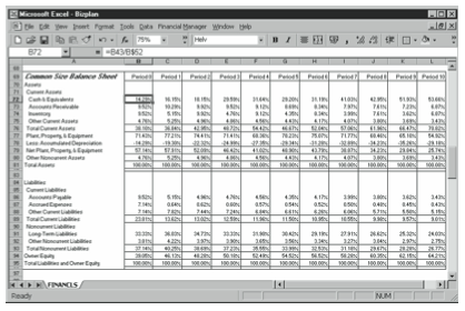
The Common Size Balance Sheet schedule has 19 rows with calculated data that express line-item amounts as percentages of the total. For the asset side of the Balance Sheet, as- sets are expressed as a percentage of the total assets. For the creditor and owner equity side of the Balance Sheet, equities are expressed as a percentage of the total liabilities and owner equity. The formulas for all rows except Total Assets and Total Liabilities and Owner Eq- uity simply convert the Balance Sheet values to percentages. For example, the Cash & Equivalents formula for the first period is:
=B43/B$52
The formula for the second period is:
=C43/C$52
and so on. All asset percentages are derived from dividing by total assets, which explains why the absolute reference to row $52 is used in all asset formulas. Similarly, the absolute reference to row $66 appears in all formulas in the liabilities and equity formulas.
The formula for the Total Assets percentage at any time is the sum of the Current Assets; the Net Plant, Property, & Equipment; and the Other Noncurrent Assets percentages. The result always equals 100 percent.
Similarly, the formula for the Total Liabilities and Owner Equity percentage at any time is the sum of the Current Liabilities, the Noncurrent Liabilities, and Owner Equity percent- ages. The result is always 100 percent.
Income Statement
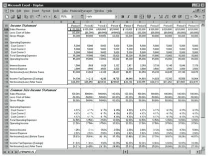
The Income Statement schedule has 13 rows of calculated data (see Figure 10-4). As in other schedules, the period identifier simply numbers the periods for which values are calculated. The first period is stored in cell C99 as the integer 1, and periods that follow are stored as the previous period plus 1. The other values in the Income Statement are calculated as described in the following paragraphs.
Sales Revenue
The Sales Revenue figures are the estimates you enter in the inputs area of the business planning starter workbook. The amount for the period is the value you enter in the inputs area of the business planning starter workbook.
Less: Cost of Sales
The Cost Of Sales figures are the Cost of Sales estimates you enter in the inputs area of the business planning starter workbook.
Gross Margin
The Gross Margin figures show the amounts left over from the sales proceeds after sub- tracting Cost of Sales. Subtracting your other expenses from the Gross Margin amount gives you your profit figure. The Gross Margin formula is Sales Revenue for the period minus Cost of Sales. For example, the formula for the first period is:
=C100+C101
The formula for the second period is:
=D100+D101
and so on. Notice that because the Cost of Sales figures are pulled into the Income State- ment schedule as negative amounts, the Gross Margin formula simply adds the Sales Rev- enue figure to the negative Cost of Sales figure.
Operating Expenses – Cost Centers 1, 2, and 3
The Operating Expenses figures for Cost Centers 1, 2, and 3 show the amount for each operating expense classification or category that you enter in the inputs area of the busi- ness planning starter workbook.
Total Operating Expenses
The Total Operating Expenses figures show the sums of the operating expenses you enter in the inputs area of the business planning starter workbook for these three operating ex- pense categories or classifications. The total for each period is the sum of the operating expenses for Cost Centers 1, 2, and 3. For example, the formula for the first period is:
=SUM(C105:C107)
The formula for the second period is:
=SUM(D105:D107)
and so on.
Operating Income
The Operating Income figures show the sales dollar amounts left after paying the Cost of Sales and the Operating Expenses. The Operating Income figures represent the amounts that go toward paying your financing expenses and income tax, and the amount that constitutes your profits.TheamountforeachperiodistheGrossMarginfigurefortheperiodminustheTotal Operating Expenses figure. For example, the formula for the first period is:
=C102-C108
The formula for the second period is:
=D102-D108
and so on.
Interest Income
The Interest Income figures show the earnings from investing the cash of the business. The amount for each period is the beginning Cash & Equivalents balance from the inputs area of the business planning starter workbook times the period yield on Cash & Equivalents. For example, the formula for the first period is:
=B43*C5
The formula for the second period is:
=C43*D5
and so on.
Interest Expense
The Interest Expense figures show the costs of using borrowed funds for operations and asset purchases. The amount for each period is the value you enter in the inputs area of the business planning starter workbook.
Net Income (Loss) Before Taxes
The Net Income (Loss) Before Taxes figures show the amount of operating income left after receiving any interest income and paying any interest expense. The amount for each period is the Operating Income figure for the period plus the Interest Income figure for the pe- riod minus the Interest Expense figure for the period. For example, the formula for the first period is:
=C109+C111-C112
The formula for the second period is:
=D109+D111-D112
and so on.
Income Tax Expenses (Savings)
The Interest Expense figures show the costs of using borrowed funds for operations and asset purchases. The amount for each period is the value you enter in the inputs area of the business planning starter workbook.
Net Income (Loss) Before Taxes
The Income Tax Expenses (Savings) figures show the income tax expenses (or savings) that use the calculated Net Income (Loss) Before Taxes figures and the Marginal Income Tax Rate figures you forecasted in the inputs area of the business planning starter workbook. Notice that the model calculates a current period savings in income taxes when there is a net loss before taxes. This might be the case when a current period loss is carried back to a prior period or when the current period loss is consolidated with the current period income of related businesses. Basically, then, the model assumes that a net loss before income taxes results in a current period tax refund—that is, an overall tax savings—because you can de- duct a loss in one business from the profits of another business. However, if a current pe- riod loss does not result in a current period income tax savings, you need to modify the formula, as described in the section “Customizing the Starter Workbook.”
The amount for each period is the Net Income (Loss) Before Taxes times the Marginal Income Tax Rate figure. For example, the formula for the first period is:
=C37*C113
The formula for the second period is:
=D37*D113
and so on.
Net Income (Loss) After Taxes
The Net Income (Loss) After Taxes figures calculate the after-tax profits of operating the business. The amount for each period is the Net Income (Loss) Before Taxes figure minus the Income Tax Expenses (Savings) figure. For example, the formula for the first period is:
=C113-C115
The formula for the second period is:
=D113-D115
and so on.
Common Size Income Statement
The Common Size Income Statement schedule lists, in income statement format, what percentage of the total sales revenue each income statement line item represents (see Figure 10-4). When you compare these percentages against those of business peers, you can see the relative financial performance of your business. Trends in the percentages over the forecasting horizon can indicate improvement or deterioration in the financial performance of your business.
The Common Size Income Statement schedule has 13 rows of calculated data that express the component line-item amount for each period as a percentage of the sales revenue fig- ure for the period. The formulas for all rows except Sales Revenue simply convert the In- come Statement values to percentages.
The Sales Revenue figures add the Cost of Sales, Total Operating Expenses, Interest In- come, Interest Expense, Income Tax Expenses (Savings), and Net Income (Loss) After Taxes percentages. The results always equal 100 percent.
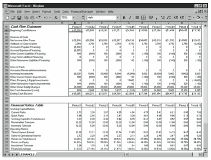
Cash Flow Statement
The Cash Flow Statement schedule has 16 rows of calculated data (see Figure 10-5). As in other schedules, a period identifier numbers the periods for which values are calculated. The first period is stored in cell C141 as integer 1. Periods that follow are stored as the pre- vious period plus 1. Other Cash Flow Statement values are calculated as described in the paragraphs that follow.
Beginning Cash Balance
The Beginning Cash Balance figures show the forecasted cash and equivalents balance at the start of each forecasting period. The starting balance is the value you enter in the in- puts area of the business planning starter workbook. For subsequent periods, the Beginning Cash Balance is the previous period’s Ending Cash Balance.
Net Income After Taxes
The Net Income After Taxes figures show the amounts calculated in the Income Statement schedule as the business profits for each forecasting period.
Addback of Depreciation
The Addback of Depreciation figures show the change in the accumulated depreciation balance for each forecasting period. Normally, this change stems from the period depreciation expense; it must be added back into the Net Income After Taxes figure because the depre- ciation expense uses no cash. The depreciation added back for each period is the value you enter in the inputs area of the business planning starter workbook as the change in accu- mulated depreciation.
Accounts Payable Financing
The Accounts Payable Financing figures show the change in the Accounts Payable balance for the period. Increases in this balance result when the cost of sales expense paid during the period is lower than the expense incurred. Decreases in this balance result when the cost of sales expense paid is higher than the expense incurred. By recognizing the changes in this account balance, the model adjusts for differences between the Income Statement’s accrual- based accounting of cost of sales expenses and the actual cash disbursements for costs of sales expenses.
The Accounts Payable Financing figure for each period is the difference between the Ac- counts Payable balance at the end of the previous period and the balance at the end of the current period. For example, the formula for the first period is:
=C57-B57
The formula for the second period is:
=D57-C57
and so on.
Accrued Expenses Financing
The Accrued Expenses Financing figures show the change in the accrued expenses balance for the period. Increases in this balance result when the operating expense paid during the period is lower than the expense incurred. Decreases in this balance result when the oper- ating expense paid during the period is higher than the expense incurred. By recognizing the changes in this account balance, the model adjusts for differences between the Income Statement’s accrual-based accounting expenses and the actual cash disbursements for op- erating expenses.
The Accrued Expenses Financing figure for each period is the difference between the Accrued Expenses balance at the end of the previous period and the balance at the end of the current period. For example, the formula for the first period is:
=C58-B58
The formula for the second period is:
=D58-C58
and so on.
Other Current Liabilities Financing
The Other Current Liabilities Financing figures show the change in the Other Current Liabilities balance for the period. This amount increases when, either directly or indirectly, cash is generated by borrowing. This amount decreases when, either directly or indirectly, cash is used to pay off short-term borrowing.
The Other Current Liabilities Financing figure for each period is the difference between the Other Current Liabilities balance at the end of the previous period and the balance at the end of the current period. For example, the formula for the first period is:
=C59-B59
The formula for the second period is:
=D59-C59
and so on.
Long-Term Liabilities Financing
The Long-Term Liabilities Financing figures show the changes in the long-term liabili- ties amount for the period. This balance increases when, either directly or indirectly, cash is generated by long-term borrowing. This amount decreases when, either directly or indi- rectly, cash is used to pay off long-term borrowing.
The Long-Term Liabilities Financing figure for each period is the difference between the Long-Term Liabilities balance at the end of the previous period and the balance at the end of the current period. For example, the formula for the first period is:
=C62-B62
The formula for the second period is:
=D62-C62
and so on.
Other Noncurrent Liabilities Financing
The Other Noncurrent Liabilities Financing figures show the changes in the Other Non- current Liabilities balance for the period. This amount increases when, either directly or indirectly, cash is generated by other long-term borrowing. This amount decreases when, either directly or indirectly, cash is used to pay off other long-term borrowing.
The Other Noncurrent Liabilities Financing figure for each period is the difference between the Other Noncurrent Liabilities balance at the end of the previous period and the balance at the end of the current period. For example, the formula for the first period is:
=C63-B63
The formula for the second period is:
=D63-C63
and so on.
Accounts Receivable Investments
The Accounts Receivable Investments figures show the change in the Accounts Receivable balance for each forecasting period. This amount increases when the sales revenue collected during the period is less than the revenue recorded. This amount decreases when the sales revenue collected during the period is more than recorded. By recognizing the changes in the account balance, the model adjusts for differences between the income statement’s accrual-based accounting of sales revenues and the actual cash collections for sales.
The Accounts Receivable Investments figure for each period is the difference between the Accounts Receivable balance at the end of the previous period and the balance at the end of the current period. For example, the formula for the first period is:
=C44-B44
The formula for the second period is:
=D44-C44
and so on.
Inventory Investments
The Inventory Investments figures show the change in the inventory balance for each fore- casting period. This amount increases when the inventory sold is less than the inventory acquired. This amount decreases when the inventory sold is more than the inventory ac- quired. By recognizing the changes in this account balance, the model recognizes the cash effects of changing inventory balances.
The Inventory Investments figure for each period is the difference between the Inventory balance at the end of the previous period and the balance at the end of the current period. For example, the formula for the first period is:
=C45-B45
The formula for the second period is:
=D45-C45
and so on.
Other Current Assets Investments
The Other Current Assets Investments figures show the changes in the Other Current Assets balance for the period. This amount increases when, either directly or indirectly, cash is used to acquire current assets. This amount decreases when indirectly or directly cash is gener- ated by converting current assets to cash.
The Other Current Assets Investments figure for each period is the difference between the Other Current Assets balance at the end of the previous period and the balance at the end of the current period. For example, the formula for the first period is:
=C46-B46
The formula for the second period is:
=D46-C46
and so on.
Plant, Property, & Equip Investments
The Plant, Property, & Equip Investments figures show the change in the Plant, Property, & Equipment balance for the period. This amount increases when, either directly or indi- rectly, cash is used to acquire plants, property and equipment. This amount decreases when, either directly or indirectly, cash is generated by converting plants, property, and equipment to cash.
The Plant, Property, & Equip Investments figure for each period is the difference between the Plant, Property, & Equipment balance at the end of the previous period and the bal- ance at the end of the current period. For example, the formula for the first period is:
=C48-B48
The formula for the second period is:
=D48-C48
and so on.
Other Noncurrent Assets Investments
The Other Noncurrent Assets Investments figures show the changes in the Other Noncur- rent Assets balance for the period. This amount increases when, either directly or indirectly, cash is used to acquire other noncurrent assets. This amount decreases when, either directly or indirectly, cash is generated by converting other noncurrent assets to cash.
The Other Noncurrent Assets Investments figure for each period is the difference between the Other Noncurrent Assets balance at the end of the previous period and the balance at the end of the current period. For example, the formula for the first period is:
=C51-B51
The formula for the second period is:
=D51-C51
and so on.
Other Owner Equity Changes
The Other Owner Equity Changes figures show the cash flows stemming from any addi- tional capital contributions made by the owners to the business or from dividends and other distributions made by the business to the owners. The Other Owner Equity Changes fig- ure is the value you enter in the inputs area of the business planning starter workbook. The Other Owner Equity Changes figures are pulled into the Uses of Cash section as negative values because a positive change in the owner equity, such as an additional capital contri- bution, such as from a stock offering, doesn’t use cash but provides cash; and a negative change in the owner equity, such as a dividend, does use cash.
Net Cash Generated (Used)
The Net Cash Generated (Used) figures show the total cash flow for each period of the forecasting horizon, based on the listed sources and uses of cash. The amount for each period is the sources of cash for the period less the uses of cash for the period. For example, the formula for the first period is:
=SUM(C145:C151)-SUM(C154:C159)
The formula for the second period is:
=SUM(D145:D151)-SUM(D154:D159)
and so on.
Ending Cash Balance
The Ending Cash Balance figures show the forecasted cash and equivalents balance at the end of each period. The balance is the Beginning Cash Balance figure for the period plus the Net Cash Generated (Used) figure for the period. For example, the formula for the first period is:
=C142+C160
The formula for the second period is:
=D142+D160
and so on.
Financial Ratios Table
The Financial Ratios Table has 11 rows of calculated data (see Figure 10-5). As in other schedules, the period identifier numbers the periods for which values are calculated. The first period is stored in cell C165 as the integer 1, and periods that follow are stored as the previous period plus 1. The other values in the Financial Ratios Table are calculated as described in the following paragraphs.
Current Ratio
The Current Ratio figures show the ratio of current assets to current liabilities. The cur- rent ratio provides one measure of a business’s ability to meet its short-term obligations. The Current Ratio figure for each period is the Total Current Assets figure from the Balance Sheet schedule divided by the Total Current Liabilities figure. For example, the formula for the first period is:
=C47/C60
The formula for the second period is:
=D47/D60
and so on.
Quick Ratio
The Quick Ratio figures show the ratio of the sum of the cash and equivalents plus the accounts receivable to the current liabilities. The quick ratio provides a more stringent measure of a business’s ability to meet its short-term financial obligations than other ratios. The Quick Ratio figure for each period is the sum of the Cash & Equivalents figure and the Accounts Receivable figure divided by the Total Current Liabilities figure. For example, the formula for the first period is:
=(C43+C44)/C60
The formula for the second period is:
=(D43+D44)/D60
and so on.
Working Capital to Total Assets
The Working Capital to Total Assets figures show the ratio of working capital (the current assets minus the current liabilities) to the total assets. The Working Capital to Total As- sets ratio is another measure of a firm’s ability to meet its financial obligations and gives an indication as to the distribution of a business’s assets into liquid and nonliquid resources.
The Working Capital to Total Assets ratio for each period is calculated by dividing the difference between the Current Assets and Current Liabilities figures by the Total Assets figure. For example, the formula for the first period is:
=(C47-C60)/C52
The formula for the second period is:
=(D47-D60)/D52
and so on.
Receivables Turnover
The Receivables Turnover figures show the ratio of sales to the accounts receivable balance. The Receivables Turnover ratio indicates the efficiency of sales collections. One problem with the measure as it’s usually applied is that both credit and cash sales might be included in the ratio denominator. Two potential shortcomings exist with this approach. First, the presence of the cash sales might make the receivables collections appear more efficient than is the case. Also, mere changes in the mix of credit and cash sales might affect the ratio, even though the efficiency of the receivables collections process has not changed.
The Receivables Turnover figure for each period is calculated by dividing the Sales Rev- enue figure for the period by the Accounts Receivable balance outstanding at the end of the period. For example, the formula for the first period is:
=C100/C44
The formula for the second period is:
=D100/D44
and so on.
Inventory Turnover
The Inventory Turnover row shows the ratio of the cost of sales to the inventory balance. The Inventory Turnover ratio calculates how long inventory is held. It can indicate depleted or excessive inventory balances. The Inventory Turnover ratio for each period is calculated by dividing the Cost of Sales figure for the period by the inventory held at the end of the period. For example, the formula for the first period is:
=-C101/C45
The formula for the second period is:
=-D101/D45
and so on.
Times Interest Earned
The Inventory Turnover row shows the ratio of the cost of sales to the inventory balance. The Inventory Turnover ratio calculates how long inventory is held. It can indicate depleted or excessive inventory balances. The Inventory Turnover ratio for each period is calculated by dividing the Cost of Sales figure for the period by the inventory held at the end of the period. For example, the formula for the first period is:
=-C101/C45
The formula for the second period is:
=-D101/D45
and so on.
Sales to Operational Assets
The Sales to Operational Assets row shows the ratio of sales of sales revenue to net plant, property, and equipment. The ratio indicates the efficiency with which a business uses its operational assets to generate sales revenue. The Sales to Operational Assets ratio for each period is the Sales Revenue figure you enter in the inputs area of the business planning starter workbook divided by the Net Plant, Property, & Equipment figure from the Balance Sheet schedule. For example, the formula for the first period is:
=C100/C50
The formula for the second period is:
=D100/D50
and so on.
Return on Total Assets
The Return on Total Assets row shows the ratio of the sum of the net income after taxes plus the interest expense to the total assets for each period. The ratio indicates the overall operating profitability of the business, expressed as a rate of return on the business assets. The formula for the first period is:
=(C16+C112)/C52
The formula for the second period is:
=(D116+D112)/D52
and so on.
Return on Equity
The Return on Equity row shows the ratio of the net income after taxes to the owner eq- uity for each period. The ratio indicates the profitability of the business as an investment of the owners. The Return on Equity ratio for each period is the Net Income (Loss) After Taxes figure from the Income Statement schedule divided by the Owner Equity figure from the Balance Sheet schedule. For example, the formula for the first period is:
=C116/C65
The formula for the second period is:
=D116/D65
and so on.
Investment Turnover
The Investment Turnover row shows the ratio of the sales revenue to the total assets. The ratio, like the Sales to Operational Assets ratio, indicates the efficiency with which a busi- ness uses its assets (in this case, its total assets) to generate sales. The Investment Turnover ratio for each period is the Sales Revenue figure you enter in the inputs area of the busi- ness planning starter workbook divided by the Total Assets figure from the Balance Sheet schedule. For example, the formula for the first period is:
=C100/C52
The formula for the second period is:
=D100/D52
and so on.
Financial Leverage
The Financial Leverage row shows the difference between the return on the owner equity and the return on the total assets. The ratio indicates the increase or decrease in an equity return as a result of borrowing. A positive value indicates an improvement in the return on owner equity by using financial leverage; a negative value indicates deterioration in the return onownerequity.TheFinancialLeveragefigureforeachperiodistheReturnonTotalAssets figure minus the Return on Equity figure. For example, the formula for the first period is:
=C176-C175
The formula for the second period is:
=D176-D175
and so on.
Leave a Reply