Figure 8-1 shows three years of sales data for a microbrewery that sells six types of beer on the West coast. The company recorded sales for each type of beer by state and by season. You can see that with the large amounts of information in the database, it’s difficult to spot trends. Creating a PivotTable allows you to see which type of beer sells best in which re- gion or during which season.
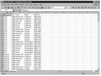
To start the PivotTable Wizard, select any cell in the database and choose the Data menu’s PivotTable And PivotChart Report command. Excel displays the dialog box shown in Figure 8-2.

If your data is in a single range on a single worksheet in the current workbook, click the Microsoft Excel List Or Database option button. Then click the PivotTable option but- ton, and click Next.
The second step of the PivotTable And PivotChart Wizard asks you to select the data you want to include in the PivotTable. Do so, and then click Next.
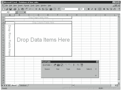
In the third and last step of the PivotTable And PivotChart Wizard, specify where you want Excel to put the PivotTable you’re creating and click Finish. As shown in Figure 8-3, Ex- cel displays the new, empty PivotTable in the location you specified. It also displays the PivotTable toolbar, which you use to lay out and edit the PivotTable.
Specifying PivotTable Layout
To begin laying out your PivotTable, use the buttons on the PivotTable toolbar to drag fields to set up row and column headings. In the example shown in Figure 8-3, you could drag the Year button to the box labeled Drop Row Fields Here and the State button to the box labeled Drop Column Fields Here. You could then drag the Sales heading to the Drop Data Items Here box. After you drag the Sales button to the Data area, Excel adds the data to the PivotTable. Figure 8-4 shows a PivotTablefilled with data.
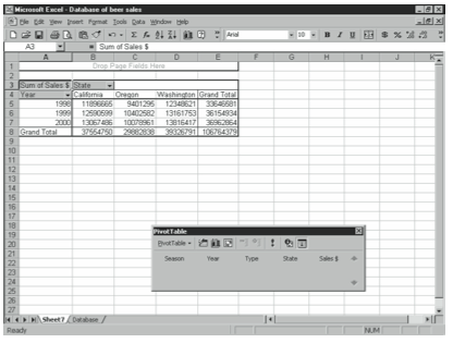
The box in the upper left corner reads Sum Of Sales $. This is because Excel assumes you want to subtotal and total sales figures. If you were to drag a label field instead of a value field into the Data area, Excel would by default count the occurrences of that label. You can change the operation performed on the data included in a PivotTable by selecting a cell in the part you want to change and clicking the PivotTable toolbar’s Field Settings button. Excel displays the PivotTable Field dialog box shown in Figure 8-5. This dialog box’s options differ slightly depending on the type of data presented in the part of the PivotTable you selected.
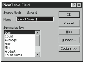
To change the operation performed on items in the field, select an item from the Summa- rize By drop-down list box and click OK. For comparative operations, click the Options button. You can then list item data as a percentage of another item, or as a difference from another item, for example.
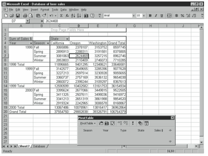
You can drag multiple fields to a heading. To add another field to a PivotTable, just drag the field’s button from the PivotTable toolbar. For example, you could drag the Season field to the right of the Year column to sort by year and then by season. Figure 8-6 shows how the PivotTable looks when you do this. To remove a field from a table, just drag the field outside the table area.
Leave a Reply