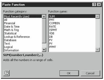
Excel provides 16 standard financial functions for making depreciation, loan payment, present value, future value, and rate of return calculations. To see which financial functions Excel provides or to see which arguments a function requires, choose the Insert menu’s Function command and then select Financial from the Function Category list box (see Figure 5-1). The first Paste Function dialog box shows the categories of functions that Excel provides—such as which financial functions are available.
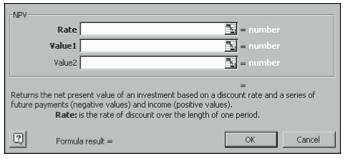
After you select a function and click OK, the second Paste Function dialog box shows which arguments are required for the function to make its calculations (see Figure 5-2).
Using the Depreciation Functions
Excel supplies five depreciation functions as part of its standard financial function set: DB, DDB, SLN, SYD, and VDB. Each of these functions apportions the cost of a long-lived asset over its estimated economic life.
DB
The DB function calculates fixed declining balance depreciation for an asset given the cost, its salvage value, estimated economic life, the accounting period for which depreciation is being calculated, and, optionally, the number of month in first year. (If you don’t include the optional month argument, Excel sets this value to 12.) The DB function uses the following syntax:
DB(cost,salvage,life,period,month)
Suppose, for example, that you must calculate the fixed declining balance depreciation for equipment that costs $50,000, lasts five years, will have a salvage value of $10,000 at the end of the fifth year, and that was placed into service in the third month of the first year. To calculate the depreciation for the first year, you use the following formula:
=DB(50000,10000,5,1,3)
The function returns the value 3437.5. To calculate the depreciation for the second year, you use the formula
=DB(50000,10000,5,2,3)
The function returns the value 12804.69
The distinguishing feature of fixed-declining balance depreciation is that it calculates depreciation at a fixed rate based on the estimated cost, salvage value, and economic life of the asset. Excel calculates this rate using the following formula:
Fixed rate=1-((salvage/cost)^(1/life))
and then rounds this value to the nearest three decimal places. To calculate the depreciation for a period, Excel multiplies the rate by the sum of the original cost less the accumulated depreciation to date.
Excel uses variations of the standard fixed-declining balance formula for the first and last periods. For the first period, Excel calculates the depreciation by using the following formula:
First-period depreciation=cost * rate * month / 12
For the last period, Excel calculates the depreciation using the following formula (which essentially just depreciates the asset down to its salvage value):
Last-period depreciation=((cost?accumulated depreciation)*rate*(12month))/12
DDB
The DDB function calculates double-declining balance depreciation for an asset given the cost, its salvage value, estimated economic life, the accounting period for which depreciation is being calculated, and, optionally, the factor at which the balance declines. (If you don’t include the optional factor argument, Excel sets this value to 2 indicating “double” declining balance.) The DDB function uses the following syntax:
DDB(cost,salvage,life,period,factor)
Suppose, for example, that you must calculate the double-declining balance depreciation for equipment that costs $50,000, lasts five years, and will have a salvage value of $10,000 at the end of the fifth year. To calculate the depreciation for the first year, you use the following formula:
=DDB(50000,10000,5,1)
The function returns the value 20000.00. To calculate the depreciation for the second year, you use the formula
=DDB(50000,10000,5,2)
The function returns the value 12000.00.
SLN
The SLN function calculates straight-line balance depreciation for an asset given the cost, its salvage value, and its estimated economic life. The DDB function uses the following syntax:
SLN(cost,salvage,life)
Suppose, for example, that you must calculate the straight-line depreciation for equipment that costs $50,000, lasts five years, will have a salvage value of $10,000 at the end of the fifth year. To calculate the depreciation for the first year, you use the following formula:
=SLN(50000,10000,5)
The function returns the value 8000.00. To calculate the depreciation for the second year, you use the same formula because straight-line depreciation is the same for each year period.
SYD
The SYD function calculates sum-of-the-years-digits depreciation for an asset given the cost, its salvage value, estimated economic life, and the accounting period for which depreciation is being calculated. The SYD function uses the following syntax:
SYD(cost,salvage,life,period)
Suppose, for example, that you must calculate the sum-of-the-years-digits depreciation for equipment that costs $50,000, lasts five years, and will have a salvage value of $10,000 at the end of the fifth year. To calculate the depreciation for the first year, use the following formula:
=SYD(50000,10000,5,1)
The function returns the value 13333.33. To calculate the depreciation for the second year, you use the formula:
=SYD(50000,10000,5,2)
The function returns the value 10666.67.
VDB
The VDB function calculates declining balance depreciation for an asset given the cost, its salvage value, estimated economic life, the starting accounting period and the ending accounting period for which depreciation is being calculated, the factor at which the balance declines, and, optionally, a switch-to-straight-line switch which is set to either TRUE or FALSE. If you set this switch to TRUE, Excel doesn’t switch to straight-line at the point when straight-line depreciation exceeds declining balance depreciation. If you set this value to FALSE, Excel does switch to straight-line. If you don’t set the optional switch-to-straightline switch to TRUE, Excel sets this value to FALSE.
The VDB function uses the following syntax:
VDB(cost,salvage,life,start period,end period,factor,switch)
Suppose, for example, that you must calculate 150% declining balance depreciation for equipment that costs $50,000, lasts five years, and will have a salvage value of $10,000 at the end of the fifth year. To calculate the depreciation for the first year, you use the following formula:
=VDB(50000,10000,5,0,1,150%)
The function returns the value 15000.00. Notice that to calculate depreciation for the first year, you set the start period to 0 and the end period to 1. To calculate the depreciation for the second year, you use the formula
=VDB(50000,10000,5,1,2,150%)
The function returns the value 10500.00. Notice that to calculate the depreciation for the second year, you set the start period to 1 and the end period to 2.
In both of the two preceding examples, Excel will automatically switch to straight-line depreciation at the point when straight-line depreciation for a period exceeds declining balance depreciation. To instruct Excel not to make this switch, you would use the following formula to calculate depreciation for the first year:
=VDB(50000,10000,5,0,1,150%,TRUE)
The word TRUE, which Excel interprets as 1, tells Excel not to switch to straight-line. To instruct Excel not to make this switch in the second year, you would use the following formula to calculate depreciation:
=VDB(50000,10000,5,1,2,150%,TRUE)
Using the Payment Functions
Excel provides five standard payment functions: IPMT, ISPMT, PMT, PPMT, and NPER. Typically, you use these functions to calculate loan payment information. You can also use them for investment annuity calculations. The paragraphs that follow describe each of these payment functions and give examples of each. As you work with each, however, keep two factors in mind:
- Be sure that you stay consistent in your period assumptions between the payment and the term and rate. In other words, if you work with monthly payments, your term and interest rate must also be expressed as monthly amounts. And if you work with annual payments, your term and interest rate must also be expressed as annual amounts.
- Note that you must use the sign of a value to indicate whether it is a cash inflow or cash outflow. An initial loan balance—assuming you’re the borrower—should be shown as a positive value because it represents a cash inflow. And loan payments as well as any balloon payments—again, assuming you’re the borrower—should be shown as negative values because they represent cash outflows. Note, too, that Excel uses signs of values in the same ways. It shows cash inflows as positive values and cash outflows as negative values.
You must keep both of these factors in mind as you work with the financial functions and especially as you work with the payment functions.
IPMT
The IPMT function calculates the interest portion of a payment given its interest rate, the period, the term (or number of payments), present value (or loan balance), future value (or balloon payment), and, optionally, the type-of-annuity switch. If you set the type-ofannuity switch to 1, Excel assumes payments occur at the beginning of the period, following the annuity due convention. If you set the annuity switch to 0 or you omit the argument, Excel assumes payments occur at the end of the period following the ordinary annuity convention.
The function uses the following syntax:
IPMT(rate,period,nper,pv,fv,type)
For example, to calculate the period interest rate for the 54th payment on a 30-year, $150,000 mortgage charging 8% annual interest, you use the following formula:
=IPMT(.08/12,54,30*12,150000,0,0)
The function returns the value -957.51. Notice that to convert the 8% annual interest to a period interest, the formula divides the annual interest rate by 12. Notice, too, that to convert the 30-year term to a term in months, the formula multiplies 30 by 12. The function returns the interest payment amount as a negative value because it reflects a cash outflow you pay.
ISPMT
Provided for compatibility with Lotus 1-2-3, the ISPMT function calculates the straightline interest portion of a payment given its interest rate, the period, the term (or number of payments), and present value (or loan balance).
ISPMT(rate,period,nper,pv)
For example, to calculate the period interest rate for the 54th payment on a 30-year, $150,000 mortgage charging 8% annual interest, you use the following formula:
=ISPMT(.08/12,54,30*12,150000)
The function returns the value –850.00. Notice that to convert the 8% annual interest to a period interest, the formula divides the annual interest rate by 12. Notice, too, that to convert the 30-year term to a term in months, the formula multiplies 30 by 12. The function returns the interest payment amount as a negative value because it reflects a cash outflow you pay.
PMT
The PMT function calculates a payment given its interest rate, the term (or number of payments), present value (or loan balance), future value (or balloon payment), and, optionally, the type-of-annuity switch. If you set the type-of-annuity switch to 1, Excel assumes payments occur at the beginning of the period, following the annuity due convention. If you set the annuity switch to 0 or you omit the argument, Excel assumes payments occur at the end of the period following the ordinary annuity convention.
The function uses the following syntax:
PMT(rate,nper,pv,fv,type)
For example, to calculate the payment on a 30-year, $150,000 mortgage charging 8% annual interest, you use the following formula:
=PMT(.08/12,30*12,150000,0,0)
The function returns the value –1100.65. Notice that to convert the 8% annual interest to a period interest, the formula divides the annual interest rate by 12. Notice, too, that to convert the 30-year term to a term in months, the formula multiplies 30 by 12. The function returns the interest payment amount as a negative value because it reflects a cash outflow you pay.
For example, to calculate the payment on a 30-year, $150,000 mortgage charging 8% annual interest that has a $25,000 balloon payment, you use the following formula:
=PMT(.08/12,30*12,150000,-25000,0)
The function returns the value -1083.87. Notice that the balloon payment argument appears as a negative value because it represents a cash outflow.
While you’ll most typically use the PMT function to calculate loan payments, you can also use it to calculate the payment required to accumulate some future value. Suppose, for example, that you want to calculate how large a contribution an employee would need to make into a 401(k) account in order to amass a $1,000,000 portfolio over 35 years. If you assume the employee will earn 9% annually, you use the following formula to make this estimate:
=PMT(.09,35,0,1000000,0)
The function returns the value –4635.84. Notice that the type switch is 0, which means that function returns the amount that must be paid at the end of the year.
If you instead want to calculate the amount that would need to be paid at the beginning of each month, you would use the following formula to make this estimate:
=PMT(.09/12,35*12,0,1000000,1)
This formula returns the value –337.40. This value is slightly less than one-twelfth of the annual, ordinary annuity value because by making payments throughout the year at the start of each month, the employee earns additional interest.
If you wanted to make the same calculation but also recognize the added fact that the employee already has $10,000 in her 401(k) account, you would use the formula:
=PMT(.09/12,35*12,-10000,1000000,1)
This formula returns the value -259.58.
PPMT
The PPMT function calculates the principal portion of a payment given its interest rate, the period, the term (or number of payments), present value (or loan balance), future value (or balloon payment), and, optionally, the type-of-annuity switch. If you set the type-ofannuity switch to 1, Excel assumes payments occur at the beginning of the period, following the annuity due convention. If you set the annuity switch to 0 or you omit the argument, Excel assumes payments occur at the end of the period following the ordinary annuity convention.
The function uses the following syntax:
PPMT(rate,period,nper,pv,fv,type)
For example, to calculate the period principal payment for the 54th payment on a 30-year, $150,000 mortgage charging 8% annual interest, you use the following formula:
=PPMT(.08/12,54,30*12,150000,0,0)
The function returns the value –143.13. Notice that to convert the 8% annual interest to a period interest, the formula divides the annual interest rate by 12. Notice, too, that to convert the 30-year term to a term in months, the formula multiplies 30 by 12. The function returns the principal payment amount as a negative value because it reflects a cash outflow you pay.
NPER
The NPER function calculates the term, or number of regular payments, on a loan or for an investment annuity given its interest rate, the payments, present value (or loan balance), future value (or balloon payment), and, optionally, the type-of-annuity switch. If you set the type-of-annuity switch to 1, Excel assumes payments occur at the beginning of the period, following the annuity due convention. If you set the annuity switch to 0 or you omit the argument, Excel assumes payments occur at the end of the period following the ordinary annuity convention.
The function uses the following syntax:
NPER(rate,pmt,pv,fv,type)
For example, to calculate the number of $1,000 monthly payments required to pay off a 9% mortgage that still has a $100,000 mortgage balance, you use the following formula:
=NPER(.09/12,-1000,100000,0,0)
The function returns the value 185.53, representing roughly 185 payments and then another roughly half payment. Notice that to convert the 9% annual interest to a period interest, the formula divides the annual interest rate by 12. Notice, too, that the payment amount, as a cash outflow, shows as a negative value while the loan balance, as an implicit cash inflow, shows as a positive value.
You can also use the NPER function to calculate investment terms. In this case, you calculate the number of payments that need to be made in order to reach some future value. Suppose, for example, that you want to calculate how many years a customer needs to contribute $2,000 to an Individual Retirement Account in order to amass a $1,000,000 portfolio. If you assume the customer will earn 9% annually and will make payments at the beginning of the year, you use the following formula to make this estimate:
=NPER(.09,-2000,0,1000000,1)
The function returns the value 43.45, indicating the $2,000 payments will need to be made for slightly more than 43 years. Notice that the type switch is 1, which means that the function returns the amount that must be paid at the beginning of the year. If you instead want to calculate the amount that would need to be paid at the beginning of each year, you would use the following formula to make this estimate:
=NPER(.09,-2000,0,1000000,0)
This formula returns the value 44.43. This value is slightly more than the annuity due value because by making payments at year-end, the customer loses interest.
If you wanted to make the same calculation but recognize the added fact that the customer already has $5,000 in his IRA account, you would use the formula:
=NPER(.09,-2000,-5000,1000000,0)
This formula returns the value 42.07.
Using the Present Value, Future Value, and Interest Rate Functions
Excel rounds out its standard financial function set with six additional functions for calculating present values, future values, and interest rates, or rates of return, including FV, IRR, MIRR, NPV, PV, and RATE.
The paragraphs that follow describe each of these functions and give examples of each. As you work with each function, let me reiterate that you need to keep two factors in mind:
- Be sure that you stay consistent in your period assumptions between the payment and the term and rate. In other words, if you work with monthly payments, your term and interest rate must also be expressed as monthly amounts. And if you work with annual payments, your term and interest rate must also be expressed as annual amounts.
- Note that you must use the sign of a value to indicate whether it is a cash inflow or cash outflow. A present value—assuming you’re the investor—should be shown as a negative value because it represents a cash outflow. And annuity amounts as well as any balloon payments—again, assuming you’re the investor—should be shown as positive if they represent cash inflows and as negative values if they represent cash outflows. Note, too, that Excel uses signs of values in the same ways. It shows cash inflows as positive values and cash outflows as negative values.
FV
The FV function calculates the future value of a loan or investment given its interest rate, the term (or number of payments), the payment, the present value (or loan balance), and, optionally, the type-of-annuity switch. If you set the type-of-annuity switch to 1, Excel assumes payments occur at the beginning of the period, following the annuity due convention. If you set the annuity switch to 0 or you omit the argument, Excel assumes payments occur at the end of the period following the ordinary annuity convention.
The function uses the following syntax:
FV(rate,nper,pmt,pv,type)
For example, to calculate the future value of a $200-a-month savings program over 25 years assuming that the investor starts with $10,000 and earns 10% annual interest, you use the following formula:
=FV(10%/12,25*12,-200,-10000,0)
The function returns the value 385936.13. Notice that to convert the 10% annual interest to a monthly interest rate, the formula divides the annual interest rate by 12. Notice, too, that to convert the 25-year term to a term in months, the formula multiplies 25 by 12. The monthly payment and initial present values show as negative amounts because they represent cash outflows. And the function returns the future value amount as a positive value because it reflects a cash inflow the investor ultimately receives.
You can also use the FV function to estimate loan balloon payment amounts. Suppose, for example, that you want to calculate the balloon payment required to pay off a $150,000 mortgage with an 8% annual interest rate after the buyer has been making $1,200-a-month payments for 10 years. You use the following formula to make this estimate:
=FV(8%/12,10*12,-1200,150000,0)
The function returns the value –113410.79. Notice that the interest rate is divided by 12 and the number of years of payments is multiplied by 12 to adjust these figures to monthly amounts. Also, notice that the monthly payment amount shows as a negative value to show it represents a cash outflow, and the initial loan balance shows as a positive value to show that it represents a cash inflow.
IRR
The IRR calculates the internal rate of return implicit in a set of cash flows given a values argument (usually a worksheet range holding the cash flow values), and, optionally, a guess at the internal rate of return value. The internal rate of return of a set of cash flows is the discount rate that produces a net present value equal to zero.
The function uses the following syntax:
IRR(values,guess)
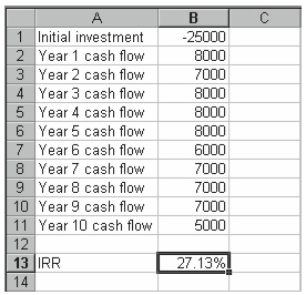
For example, if you store the cash flows from an investment into worksheet like the one shown in Figure 5-3, you can use the following formula to calculate the investment’s internal rate of return:
=IRR(B1:B11)
The function returns the value 27.13%.
You’ll want to consider several things if you use the IRR function:
- The values argument needs to contain at least one positive value and at least one negative value. If your investment doesn’t meet at least these requirements, it doesn’t look enough like an investment to be measured by the IRR function.
- The order of the cash flows in the values argument should reflect their actual order: the first cash flow first, the second cash flow second, and so on.
- The cash flow periods must be consistent. In Figure 5-3, for example, the cash flow periods are all years—and that works. But you couldn’t mix and match annual and monthly cash flow in such a values range.
Although you aren’t required to use a guess argument because Excel assumes an initial guess of 10%, you may need to do so. Excel attempts to solve the IRR function’s equation iteratively. If the equation can’t be solved after 20 attempts to within .00001, the function returns the #NUM error value. Excel usually succeeds if the internal rate of return value is close to typical returns (say, between –10% and 30%), but it sometimes has trouble with returns that are outside this range. And in this case, if you supply a guess argument that’s close to the actual internal rate of return value, you in effect help Excel start its search close to its destination.
One consideration in using the IRR function is that theoretically it doesn’t actually have a single correct solution. In practice, a set of cash flows will sometimes have as many valid internal rates of return as there are sign changes.
In the worksheet shown in Figure 5-3, only one cash flow sign change occurs (from negative cash flow at the start of the investment to positive cash flow in year one). In a case like that shown in Figure 5-4, however, the IRR function can actually return two valid internal rate of return values because there are two sign changes—one between the initial investment and the first-year cash flow and another between the first-year cash flow and the second-year cash flow.
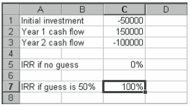
If you don’t supply a guess, Excel calculates the internal rate of return to be equal to zero. If you happen to supply a large guess value—the worksheet in Figure 5-4 uses a guess equal to 50%—Excel calculates the internal rate of return to be equal to 100%. Both calculations are right. What’s happening is that Excel finds the calculation result that’s closest to your guess or its guess.
MIRR
The MIRR function calculates the modified internal rate of return implicit in a set of cash flows given the cash flow values (usually a worksheet range holding the cash flow values), the finance rate, and the reinvestment rate. This rate of return calculation differs from the IRR function’s calculation (described in the preceding paragraphs) in two ways: it assumes that interim cash inflows are reinvested at some specified rate of return, and it assumes that interim cash outflows are funded by borrowing at some specified interest rate.
The function uses the following syntax:
MIRR(values,finance rate,reinvest rate)
For example, if you store the cash flows from an investment into a worksheet such as the one shown in Figure 5-5, you will borrow money at 10% to pay for the first year’s cash outflow, and then you will reinvest the cash flows in years two through ten at 12%. You can use the following formula to calculate the investment’s modified rate of return:
=MIRR(C1:C11,.1,.12)
The function returns the value 12.43%.
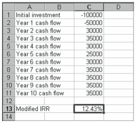
While it’s not clear from the Excel documentation that this is the case, MIRR discounts any interim cash outflows back to an equivalent present value using the finance rate and compounds any interim cash inflows out to an equivalent future value amount using the reinvestment rate. The modified internal rate of return value, then, is the rate that equates the initial present value of the cash outflows with the future value of the cash inflows.
As with the IRR function, you’ll want to consider several factors if you use the MIRR function:
- The values argument needs to contain at least one positive value and at least one negative value. If your investment doesn’t meet at least these requirements, it doesn’t look enough like an investment to be measured by the MIRR function.
- The order of the cash flows in the values argument should reflect their actual order: the first cash flow first, the second cash flow second, and so on.
- The cash flow periods must be consistent. In Figure 5-5, for example, the cash flow periods are all years.
NPV
The NPV function calculates the net present value of a set of cash flows given the discount rate and the cash flow values (usually a worksheet range holding the cash flow values). If you are using the NPV function to compare alternative investments, the investment opportunity with the largest NPV is the one that generates the largest profit in absolute, present value terms.
The function uses the following syntax:
NPV(rate,values)
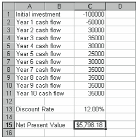
For example, if you store the cash flows from an investment into a worksheet such as the one shown in Figure 5-6 (with the same cash flows as those shown in Figure 5-5), you can use the following formula to calculate the investment’s modified rate of return:
=NPV(C13,C1:C11)
The function returns the value $5,798.18.
You’ll want to consider several factors if you use the NPV function:
- The NPV function assumes that the first cash flow occurs immediately, or at what’s sometimes referred to as period 0.
- The rate argument needs to be the discount rate for the time period used to calibrate cash flows. In other words, if you’re using monthly cash flows, your discount rate needs to be a monthly rate.
- The values argument can include more than one cell or range. You can, for example, use the NPV function NPV(.1,A1,A2,A3,A4:A8).
- The order of the cash flows in the values argument should reflect their actual order: the first cash flow first, the second cash flow second, and so on.
- The NPV function recognizes empty cells, or cells that contain text labels are zeroes in its calculations. However, if you include an array, any empty cells or cells containing text labels are ignored.
PV
The PV function calculates the present value of an annuity, or future value, given the periodic rate, number of periods, payment, future value (or balloon payment), and, optionally, the type-of-annuity switch. If you set the type-of-annuity switch to 1, Excel assumes payments occur at the beginning of the period, following the annuity due convention. If you set the annuity switch to 0 or you omit the argument, Excel assumes payments occur at the end of the period following the ordinary annuity convention.
The function uses the following syntax:
PV(rate,nper,pmt,fv,type)
For example, if you want to estimate the outstanding balance on a mortgage loan that charges 8%, requires two hundred more $1,000-a-month payments, and also requires a $10,000 balloon payment, you can use the following formula:
=PV(.08/12,200,-1000,-10000)
The function returns the value $112,932.75.
RATE
The Rate function calculates the interest rate implicit in a set of loan or investment terms given the number of periods, the payment, the present value, the future value, and, optionally, the type-of-annuity switch, and also optionally, an interest-rate rate.
If you set the type-of-annuity switch to 1, Excel assumes payments occur at the beginning of the period, following the annuity due convention. If you set the annuity switch to 0 or you omit the argument, Excel assumes payments occur at the end of the period following the ordinary annuity convention.
The function uses the following syntax:
RATE(nper,pmt,pv,fv,type,guess)
For example, suppose you want to calculate the implicit interest rate on a car lease that requires five years of $250-a-month payments (occurring as an annuity due) and also a $15,000 balloon payment. To do this, assuming you want to start with a guess of 10%, you can use the following formula:
=RATE(5*12,-250,20000,-15000,1)
The function returns the value .95%, which is a monthly interest rate of just less than 1%. If you annualize this monthly rate by multiplying it by 12, you get an equivalent annual interest rate of 11.41%.
Leave a Reply